Posted by Daniel Ellis, TensorFlow Engineer
Note: This blog post is aimed at TensorFlow developers who want to learn the details of how graphs and models are stored. If you are new to TensorFlow, you should check out the TensorFlow Basics guides before reading this article.
TensorFlow can run models without the original Python objects, as demonstrated by TensorFlow Serving and TensorFlow Lite, or when you download a trained model from TensorFlow Hub.
Models and layers can be loaded from this representation without actually making an instance of the Python class that created it. This is desired in situations where you do not have (or want) a Python interpreter, such as serving at scale or on an edge device, or in situations where the original Python code is not available.
Saved models are represented by two separate, but equally important, parts: the graph, which describes the fixed computation described in code, and the weights, which are the dynamic parameters you trained during training. If you aren’t already familiar with this and @tf.function, you should check out the Introduction to graphs and functions guide as well as the section on saving in the modules, layers, and models guide.
From a code standpoint, functions decorated with @tf.function create a Python callable; in the documentation we refer to these as polymorphic functions, as they are Python callables that can take a variety argument signatures. Each time you call a @tf.function with a new argument signature, TensorFlow traces out a new graph just for that set of arguments. This new graph is then added as a “concrete function” to the callable. Thus, a saved model can be one or more subgraphs, each with a different signature.
A SavedModel is what you get when you call tf.saved_model.save(). Saved models are stored as a directory on disk. The file, saved_model.pb,within that directory, is a protocol buffer describing the functional tf.Graph.
In this blog post, we’ll take a look inside this protobuf and see how function signature serialization and deserialization works under the hood. After reading this, you’ll have a greater appreciation for what functions and signatures before, which can help you load, modify, or optimize saved models.
Background
There are a total of five places inputs to functions are defined in the saved model protobuf. It can be tough to understand and remember what each of these does. This post intends to inventory each of these definitions and what they’re used for. It also goes through a basic example illustrating what a simple model looks like after serialization.
The actual APIs you use will always be carefully versioned (as they have been since 2016), and the models themselves will conform to the version compatibility guide. However, the material in this document lays out a snapshot of the existing state of things. Any links to code will include point-in-time revisions so as not to drift out of date. As with all non-documented implementation details, these details are subject to change in the future.
We’ll occasionally use the term “signatures” to talk about the general concept of describing function inputs (e.g. in the title of this document). In this sense, we will be referring not just to TensorFlow’s specific concept of signatures, but all of the ways TensorFlow defines and validates inputs to functions. Context should make the meaning clear.
What This Is Not About
This document is not intended to describe how signatures or functions work from a user perspective. It is intended for TensorFlow developers working on the internals of TensorFlow. Likewise, this document does not make a statement of the way things “should” be. It aims to simply document the way things are.
Overview of Signature Definitions
There are five protos that store definitions of function inputs in one manner or another. Their names and code locations, as well as their paths within the saved model proto, are as follows:
Proto messages, and their location in SavedModel
- FunctionDef: meta_graphs -> graph_def -> library -> function
- SignatureDef: meta_graphs -> signature_def
- SavedFunction: meta_graphs -> object_graph_def -> nodes -> kind -> function
- SavedBareConcreteFunction: meta_graphs -> object_graph_def -> nodes -> kind -> bare_concrete_function
- SavedConcreteFunction: meta_graphs -> object_graph_def -> concrete_functions
FunctionDef
Of the five definitions discussed in this document, FunctionsDefs are the most core to execution. When loading a saved model, these function definitions are registered in the function library of the runtime and used to create ConcreteFunctions. These functions can then be executed via PartitionedCall or TFE_Py_Execute.
This is where the actual nodes describing execution are defined, as well as what the inputs and outputs to the function are.
SignatureDef
SignatureDefs are generated from signatures passed into @tf.function. We do not save the signature’s TensorSpecs directly, however. Instead, when saving, we call the underlying function using the TensorSpecs in order to generate a concrete function. From there, we inspect the generated concrete function to get the inputs and outputs, storing them on the SignatureDef.
On the loading side,SignatureDefs are essentially ignored. They are primarily used in v1 or C++, where the developer loading the model can inspect the returned SignatureDef protos directly. This allows them to use their desired signature name to lookup the placeholder and output names needed for execution.
These input and output names can then be passed into feeds and fetches when calling Session.run in TensorFlow V1 code.
SavedFunction
SavedFunction is one of the many types of SavedObjects in the nodes list of the ObjectGraphDef. SavedFunctions are restored into a RestoredFunctions at load time. Like all nodes in this list, they are then attached to the returned model via the hierarchy defined by the children ObjectReference field.
SavedFunction’s main purpose is polymorphism. SavedFunctions support polymorphism by specifying a number of concrete function names defined in the function library above (via FunctionDef). At call time, we iterate through the concrete function names to find the first whose signature matches. If we find a match, we call it; if not, we throw an exception.
There is one more bit of complexity. When a RestoredFunction is called with a particular set of arguments, a new concrete function is created whose sole purpose is to call the matching concrete function. This is done using restored_function_body under the hood and is where the logic lives to find the appropriate concrete function.
This is invisible in the SavedModel proto, but these extra concrete functions are registered at call time in the runtime’s function library just as the other function library functions are.
The second purpose of SavedFunction is to update the FunctionSpec of all associated ConcreteFunctions using the FunctionSpec stored on the SavedFunction. This function spec is used at call time to
- validate passed in structured arguments, and
- convert structured arguments into flat ones needed for calling the underlying concrete function.
SavedBareConcreteFunction
Similar to SavedFunctions, SavedBareConcreteFunctions are used to update a
specific concrete function’s arguments and function spec. This is done here. Unlike SavedFunctions, they only reference a single specific concrete function.
In practice, SavedBareConcreteFunctions are commonly attached to and accessed via the signatures map (i.e. the signatures attribute on the loaded object). The underlying concrete functions they modify, in this case, are signature_wrapper functions. This wrapping is done to format the output in the way v1 expects (i.e. a dictionary of tensors). Similar to restored_function_body concrete functions, and other than restructuring the output, these concrete functions do nothing but call their associated concrete functions.
SavedConcreteFunction
SavedConcreteFunction objects are not SavedObjectGraph nodes. They are stored in a map directly on the SavedObjectGraph. These objects reference a specific, already-registered concrete function — the key in the map is that concrete function’s registered name.
These objects serve two purposes. The first is handling function “captures” via
the bound_inputs field. Captured variables are those a function reads or modifies that were not explicitly passed in when calling into the function. Since functions in the function library do not have a concept of captured variables, any variables used by the function must be passed in as an argument. bound_inputs stores a list of node IDs that should be passed in to the underlying ConcreteFunction when called. We set this up here.
The second purpose, and similar to SavedFunction and SavedBareConcreteFunction, is modifying the existing concrete function’s FuncGraph structured inputs and outputs. This also is used for argument validation. The setup for this is done here.
Example Walkthrough
A simple example may help illustrate all of this with more clarity. Let’s make a basic model and take a look at the subsequent generated proto to get a better feel for what’s going on.
Basic Model
class ExampleModel(tf.Module):

  @tf.function(input_signature=[tf.TensorSpec(shape=(), dtype=tf.float32)])
  def capture_fn(self, x):
    if not hasattr(self, 'weight'):
      self.weight = tf.Variable(5.0, name='weight')
    self.weight.assign_add(x * self.weight)
    return self.weight

  @tf.function
  def polymorphic_fn(self, x):
    return tf.constant(3.0) * x

model = ExampleModel()
model.polymorphic_fn(tf.constant(4.0))
model.polymorphic_fn(tf.constant([1.0, 2.0, 3.0]))
tf.saved_model.save(
    model, "/tmp/example-model", signatures={'capture_fn': model.capture_fn})
This model contains the basis for most of the complexity we’ll need to fully explore the intricacies of saving and signatures. This will allow us to look at functions with and without signatures, with and without captures, and with and without polymorphism.
Function with Captures
Let’s start by looking at our function with captures, capture_fn. We can see we have a concrete function defined in the function library, as expected:
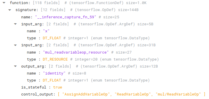 |
A FunctionDef located in FunctionDefLibrary of MetaGraphDef.graph_def |
Note the expected float input, "x", as well as the additional captured argument, "mul_readvariableop_resource". Since this function has a capture, we should see a variable being referenced in the bound_inputs field of one of our SavedConcreteFunctions:
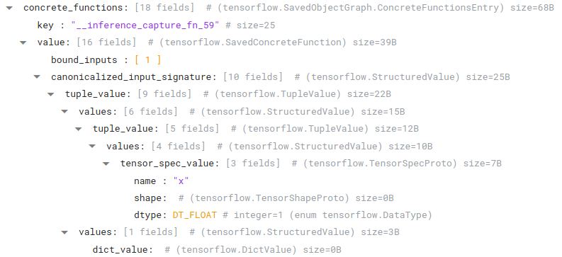 |
A SavedConcreteFunction located in the concrete_functions map of the ObjectGraphDef |
Indeed, we can see bound_inputs refers to node 1, which is a SavedVariable with the name and dtype we expect:
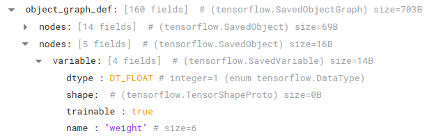 |
A SavedVariable located in ObjectGraphDef.nodes |
Note that we also are storing on canonicalized_input_signature additional data that will be used to modify the concrete function. The key of this object, "__inference_capture_fn_59", is the same name as the concrete function registered in our function library.
Since we’ve specified a signature, we should also see a SavedBareConcreteFunction:
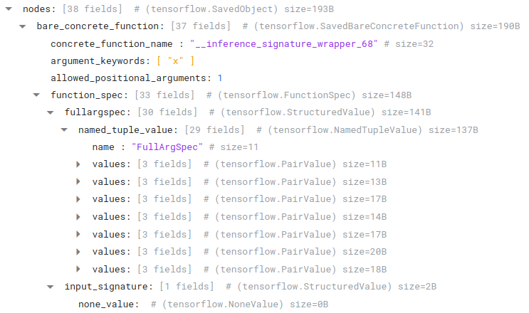 |
A SavedBareConcreteFunction located in ObjectGraphDef.nodes |
As discussed above, we use the function spec and argument information to modify the underlying concrete function. But what’s up with the "__inference_signature_wrapper_68" name? And how does this fit in with the rest of the code?
First, note that this is the fifth (5) node in the node list. This will come up again shortly.
Let’s start by looking at the nodes list. If we start at the first node in the nodes list, we’ll see a "signatures" node attached as a child:
 |
A SavedUserObject located in ObjectGraphDef.nodes |
If we look at node 2, we’ll see this node is a signature map that references one final node: node 5, our BareConcreteSavedFunction.
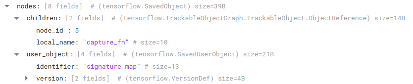 |
A SavedUserObject located in ObjectGraphDef.nodes |
Thus, when we access this function via model.signatures["capture_fn"], we will actually be calling into this intermediate signature wrapper function first.
And what does that function, "__inference_signature_wrapper_68", look like?
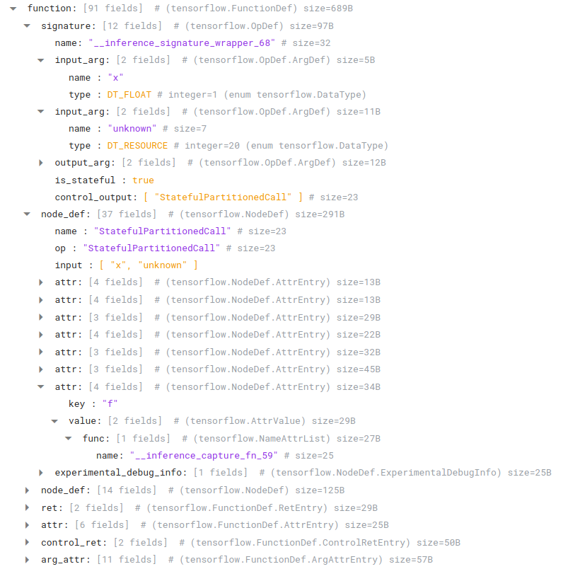 |
A FunctionDef located in FunctionDefLibrary of MetaGraphDef.graph_def |
It takes the arguments we expect, and makes a call out to… "__inference_capture_fn_59", our original function! Just as we expect.
But wait… what happens if we don’t access our function via model.signatures["capture_fn"]? After all, we should be able to call it directly via model.capture_fn.
Notice above, we had a child on the top level object named "capture_fn" with a node_id of 3. If we look at node 3, we’ll see a SavedFunction object that references our original concrete function with no signature wrapper intermediary:
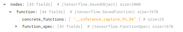 |
A SavedFunction located in ObjectGraphDef.nodes |
Again, the function spec is used to modify the function spec of our concrete function, "__inference_capture_fn_59". Notice also that concrete_functions here is a list. We only have one item right now, but this will come up again when we take a look at our polymorphic function example.
Now, we’ve fully mapped essentially everything needed for execution of this function, but we have one last thing to look at: SignatureDef. We’ve defined a signature, so we expect a SignatureDef to be defined:
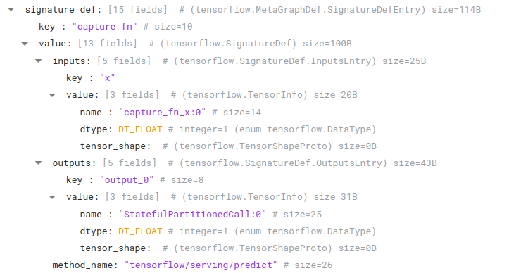 |
A SignatureDef located in the MetaObjectGraph.signature_def map |
This is very important for loading in v1 and C++ for serving. Note those funky names: "capture_fn_x:0" and "StatefulPartitionedCall:0". To call this function in v1, we need a way to map our nice argument names to the actual graph placeholder names for passing in as feeds and fetches (and doing validation, if we wish). Looking at this SignatureDef allows us to do just that.
Polymorphic Functions
We’re not quite done yet. Let’s take a look at our polymorphic function. We won’t repeat everything, since a lot of it is the same. We won’t have any signature wrapper functions or signature defs, since we skipped the signature on this one. Let’s look at what’s different.
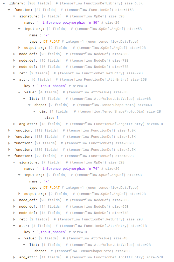 |
A FunctionDef located in FunctionDefLibrary of MetaGraphDef.graph_def |
For one, we now have two concrete functions registered in the function library, each with slightly different input shapes.
We also have two SavedConcreteFunction modifiers:
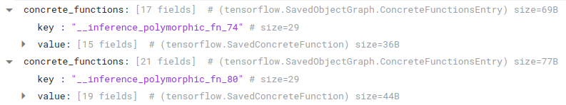 |
Two SavedConcreteFunctions located in the concrete_functions map of the ObjectGraphDef |
And finally, we can see our SavedFunction references two underlying concrete functions instead of one:
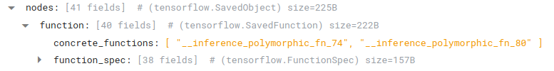 |
A SavedFunction located in ObjectGraphDef.nodes |
The function spec here will be attached to both of these concrete functions at load time. When we call our SavedFunction, it will use the arguments we pass in to find the correct concrete function and execute it.
Next Steps
You should now be an expert on how functions and their signatures are saved at a code level. Remember, what’s described in this blog post is how the code works right now. For updated code and examples in the future, see the official documentation on tensorflow.org.
Speaking of documentation, if you want a fast introduction to the basic APIs for saved models, you should introductory articles on how the APIs for functions and modules are traced and saved. For experts, don’t miss this detailed guide on SavedModel itself, as well as a complete discussion of autograph.
And finally, if you do any exciting or useful protobuf surgery, share with us on Twitter. Thanks for reading this far!