Posts in category: Tensorflow

Posted by Andrea Skolik, Volkswagen AG and Leiden University

In early March, Google released TensorFlow Quantum (TFQ) together with the University of Waterloo and Volkswagen AG. TensorFlow Quantum is a software framework for quantum machine learning (QML) which allows researchers to jointly use functionality from Cirq and TensorFlow. Both Cirq and TFQ are aimed at simulating noisy intermediate-scale quantum (NISQ) devices that are currently available, but are still in an experimental stage and therefore come without error correction and suffer from noisy outputs.

In this article, we introduce a training strategy that addresses vanishing gradients in quantum neural networks (QNNs), and makes better use of the resources provided by a NISQ device. If you’d like to play with the code for this example yourself, check out the notebook on layerwise learning in the TFQ research repository, where we train a QNN on a simulated quantum computer!

Quantum Neural Networks

Training a QNN is not that much different from training a classical neural network, just that instead of optimizing network weights, we optimize the parameters of a quantum circuit. A quantum circuit looks like the following:

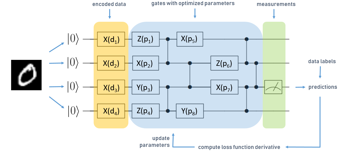
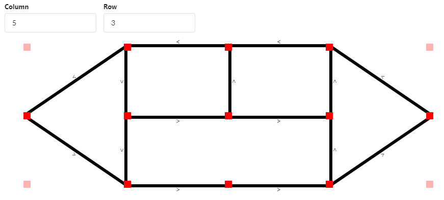
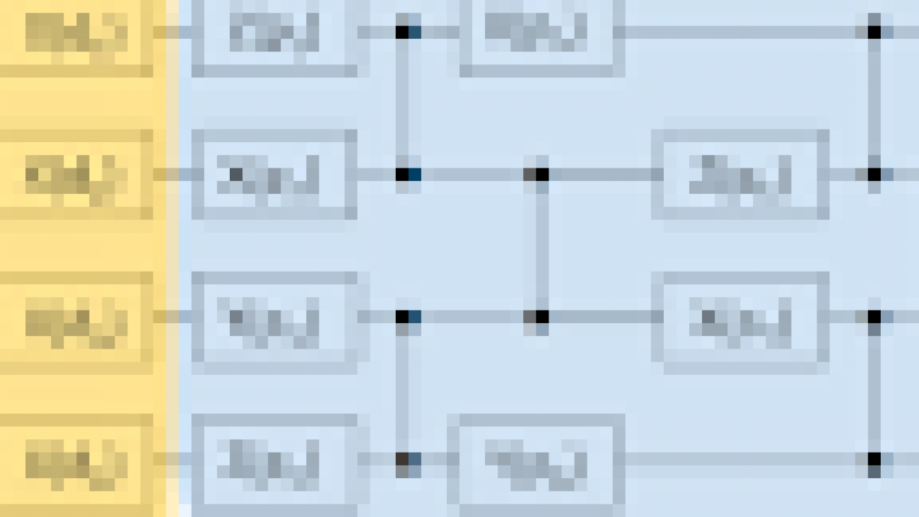
Simplified QNN for a classification task with four qubits

The circuit is read from left to right, and each horizontal line corresponds to one qubit in the register of the quantum computer, each initialized in the zero state. The boxes denote parametrized operations (or “gates”) on qubits which are executed sequentially. In this case we have three different types of operations, X, Y, and Z. Vertical lines denote two-qubit gates, which can be used to generate entanglement in the QNN – one of the resources that lets quantum computers outperform their classical counterparts. We denote one layer as one operation on each qubit, followed by a sequence of gates that connect pairs of qubits to generate entanglement.

The figure above shows a simplified QNN for learning classification of MNIST digits.

First, we have to encode the data set into quantum states. We do this by using a data encoding layer, marked orange in the figure above. In this case, we transform our input data into a vector, and use the vector values as parameters d for the data encoding layers’ operations. Based on this input, we execute the part of the circuit marked in blue, which represents the trainable gates of our QNN, denoted by p.

The last operation in the quantum circuit is a measurement. During computation, the quantum device performs operations on superpositions of classical bitstrings. When we perform a readout on the circuit, the superposition state collapses to one classical bitstring, which is the output of the computation that we get. The so-called collapse of the quantum state is probabilistic, to get a deterministic outcome we average over multiple measurement outcomes.

In the above picture, marked in green, we perform measurements on the third qubit and use these to predict labels for our MNIST examples. We compare this to the true data label and compute gradients of a loss function just like in a classical NN. These types of QNNs are called “hybrid quantum-classical”, as the parameter optimization is handled by a classical computer, using e.g. the Adam optimizer.

Vanishing gradients, aka barren plateaus

It turns out that QNNs also suffer from vanishing gradients, just like classical NNs. Since the reason for vanishing gradients in QNNs is fundamentally different from classical NNs, a new term has been adopted for them: barren plateaus. Covering all details of this important phenomenon is out of the scope of this article, so we refer the interested reader to the paper that first introduced barren plateaus in QNN training landscapes or this tutorial on barren plateaus on the TFQ site for a hands-on example.

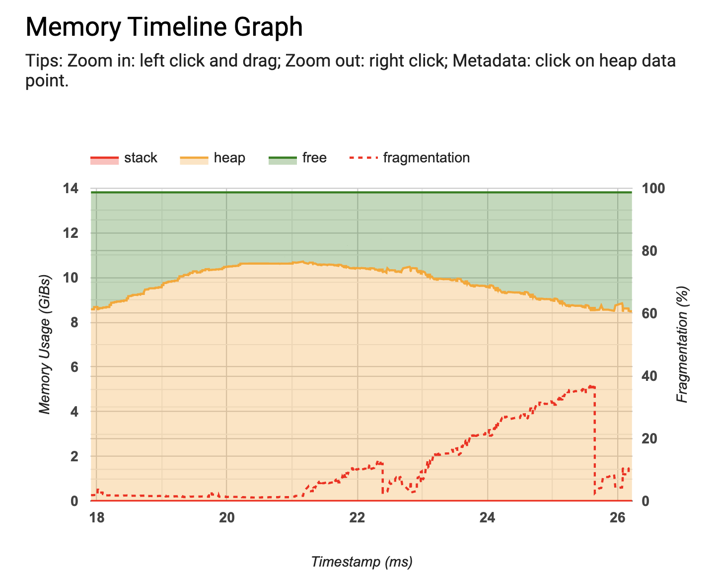
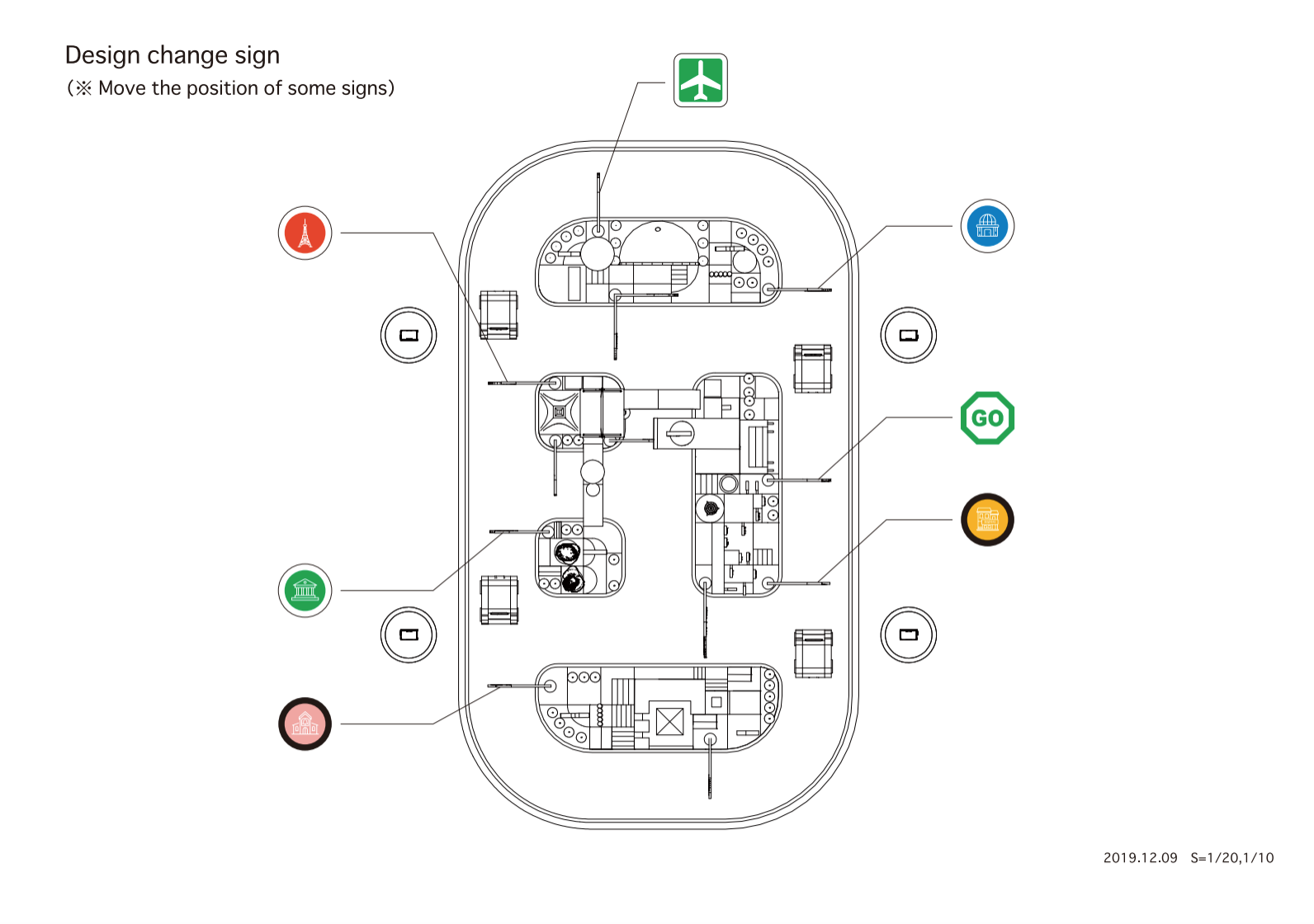
In short, barren plateaus occur when quantum circuits are initialized randomly – in the circuit illustrated above this means picking operations and their parameters at random. This is a fundamental problem for training parametrized quantum circuits, and gets worse as the number of qubits and the number of layers in a circuit grows, as we can see in the figure below.

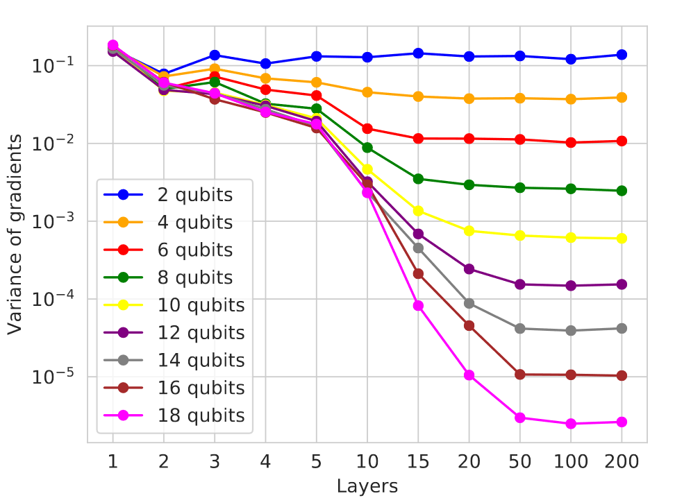
Variance of gradients decays as a function of the number of qubits and layers in a random circuit

For the algorithm we introduce below, the key thing to understand here is that the more layers we add to a circuit, the smaller the variance in gradients will get. On the other hand, similarly to classical NNs, the QNN’s representational capacity also increases with its depth. The problem here is that in addition, the optimization landscape flattens in many places as we increase the circuit’s size, so it gets harder to find even a local minimum.

Remember that for QNNs, outputs are estimated from taking the average over a number of measurements. The smaller the quantity we want to estimate, the more measurements we will need to get an accurate result. If these quantities are much smaller compared to the effects caused by measurement uncertainty or hardware noise, they can’t be reliably determined and the circuit optimization will basically turn into a random walk.

To successfully train a QNN, we have to avoid random initialization of the parameters, and also have to stop the QNN from randomizing during training as its gradients get smaller, for example when it approaches a local minimum. For this, we can either limit the architecture of the QNN (e.g. by picking certain gate configurations, which requires tuning the architecture to the task at hand), or control the updates to parameters such that they won’t become random.

Layerwise learning

In our paper Layerwise learning for quantum neural networks, which is joint work by the Volkswagen Data:Lab (Andrea Skolik, Patrick van der Smagt, Martin Leib) and Google AI Quantum (Jarrod R. McClean, Masoud Mohseni), we introduce an approach to avoid initialization on a plateau as well as the network ending up on a plateau during training. Let’s look at an example of layerwise learning (LL) in action, on the learning task of binary classification of MNIST digits. First, we need to define the structure of the layers we want to stack. As we make no assumptions about the learning task at hand, we choose the same layout for our layers as in the figure above: one layer consists of random gates on each qubit initialized with zero, and two-qubit gates which connect qubits to enable generation of entanglement.

We designate a number of start layers, in this case only one, which will always stay active during training, and specify the number of epochs to train each set of layers. Two other hyperparameters are the number of new layers we add in each step, and the number of layers that are maximally trained at once. Here we choose a configuration where we add two layers in each step, and freeze the parameters of all previous layers, except the start layer, such that we only train three layers in each step. We train each set of layers for 10 epochs, and repeat this procedure ten times until our circuit consists of 21 layers overall. By doing this, we utilize the fact that shallow circuits produce larger gradients compared to deeper ones, and with this avoid initializing on a plateau.

This provides us with a good starting point in the optimization landscape to continue training larger contiguous sets of layers. As another hyperparameter, we define the percentage of layers we train together in the second phase of the algorithm. Here, we choose to split the circuit in half, and alternatingly train both parts, where the parameters of the inactive parts are always frozen. We call one training sequence where all partitions have been trained once a sweep, and we perform sweeps over this circuit until the loss converges. When the full set of parameters is always trained, which we will refer to as “complete depth learning” (CDL), one bad update step can affect the whole circuit and lead it into a random configuration and therefore a barren plateau, from which it cannot escape anymore.

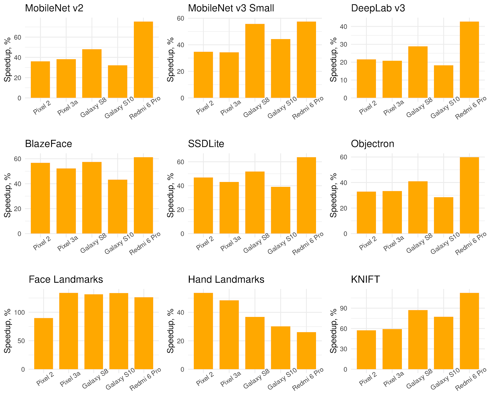
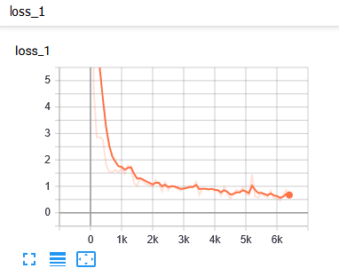
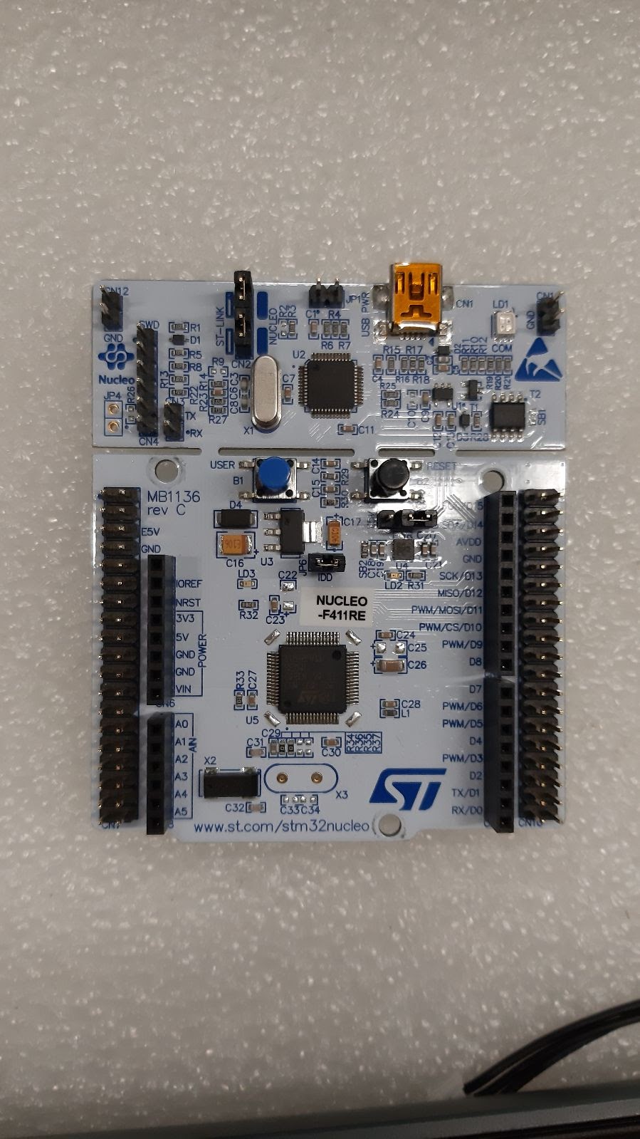
Let’s compare our training strategy to CDL, which is one of the standard techniques used to train QNNs. To get a fair comparison, we use exactly the same circuit architecture as the one generated by the LL strategy before, but now update all parameters simultaneously in each step. To give CDL a chance to train, we optimize the parameters with zero instead of randomly. As we don’t have access to a real quantum computer yet, we simulate the probabilistic outputs of the QNN, and choose a relatively low value for the number of measurements that we use to estimate each prediction the QNN makes – which is 10 in this case. Assuming a 10kHZ sampling rate on a real quantum computer, we can estimate the experimental wall-clock time of our training runs as shown below:

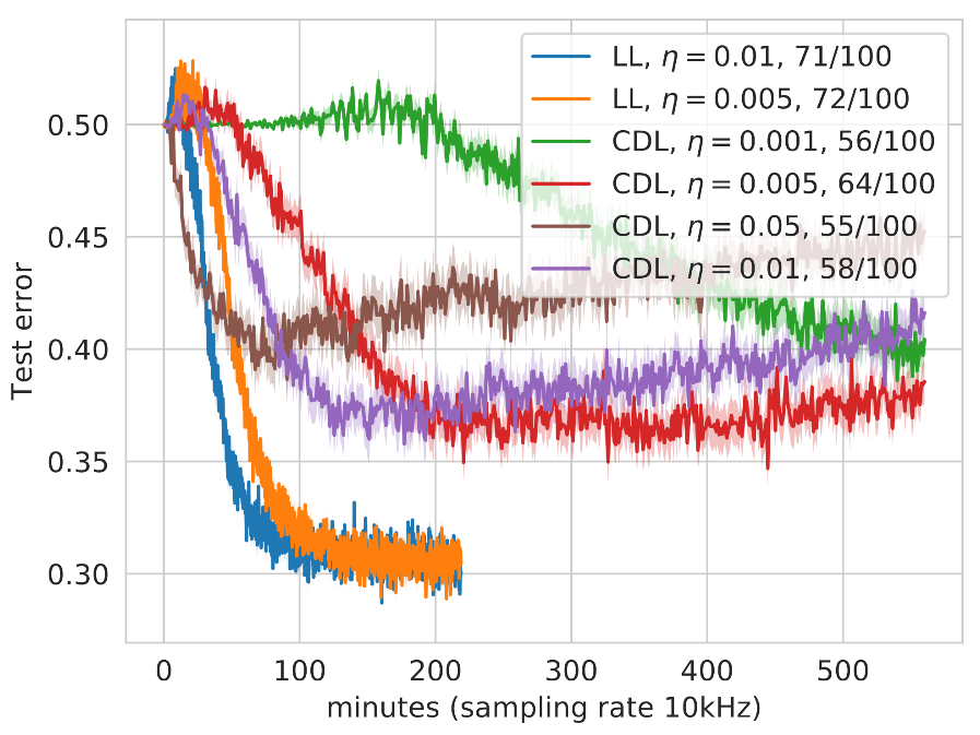
Comparison of layerwise- and complete depth learning with different learning rates η. We trained 100 circuits for each configuration, and averaged over those that achieved a final test error lower than 0.5 (number of succeeding runs in legend).

With this small number of measurements, we can investigate the effects of the different gradient magnitudes of the LL and CDL approaches: if gradient values are larger, we get more information out of 10 measurements than for smaller values. The less information we have to perform our parameter updates, the higher the variance in the loss, and the risk to perform an erroneous update that will randomize the updated parameters and lead the QNN onto a plateau. This variance can be lowered by choosing a smaller learning rate, so we compare LL and CDL strategies with different learning rates in the figure above.

Notably, the test error of CDL runs increases with the runtime, which might look like overfitting at first. However, each curve in this figure is averaged over many runs, and what is actually happening here is that more and more CDL runs randomize during training, unable to recover. In the legend we show that a much larger fraction of LL runs achieved a classification error on the test set lower than 0.5 compared to CDL, and also did it in less time.

In summary, layerwise learning increases the probability of successfully training a QNN with overall better generalization error in less training time, which is especially valuable on NISQ devices. For more details on the implementation and theory of layerwise learning, check out our recent paper!

If you’d like to learn more about quantum computing and quantum machine learning in general, there are some additional resources below:

• Quirk: a drag-and-drop quantum circuit simulator with nice visualizations
• Quantum Intuition on YouTube, which has many helpful video tutorials
• The TensorFlow Quantum whitepaper, for a deep dive into the theory behind QNNs
• The book Quantum Computing: An Applied Approach which covers theory as well as hands-on examples with code

Read More

Posted by Josh Gordon, Developer Advocate

A new HarvardX TinyML course on edX.org

Prof. Vijay Janapa Reddi of Harvard, the TensorFlow Lite Micro team, and the edX online learning platform are sharing a series of short TinyML courses this fall that you can observe for free, or sign up to take and receive a certificate. In this article, I’ll share a bit about TinyML, what you can do with it, and the upcoming HarvardX program.

About TinyML

TinyML is one of the fastest-growing areas of Deep Learning. In a nutshell, it’s an emerging field of study that explores the types of models you can run on small, low-power devices like microcontrollers.

TinyML sits at the intersection of embedded-ML applications, algorithms, hardware and software. The goal is to enable low-latency inference at edge devices on devices that typically consume only a few milliwatts of battery power. By comparison, a desktop CPU would consume about 100 watts (thousands of times more!). Such extremely reduced power draw enables TinyML devices to operate unplugged on batteries and endure for weeks, months and possibly even years — all while running always-on ML applications at the edge/endpoint.

TinyML powering a simple speech recognizer. Learn how to build your own here.

Although most of us are new to TinyML, it may surprise you to learn that TinyML has served in production ML systems for years. You may have already experienced the benefits of TinyML when you say “OK Google” to wake up an Android device. That’s powered by an always-on, low-power keyword spotter, not dissimilar in principle from the one you can learn to build here.

The difference now is that TinyML is becoming rapidly more accessible, thanks in part to TensorFlow Lite Micro and educational resources like this upcoming HarvardX course.

TinyML unlocks many applications for embedded ML developers, especially when combined with sensors like accelerometers, microphones, and cameras. It is already proving useful in areas such as wildlife tracking for conservation and detecting crop diseases for agricultural needs, as well as predicting wildfires.

TinyML can also be fun! You can develop smart game controllers such as controlling a T-Rex dinosaur using a neural-network-based motion controller or enable a variety of other games. Using the same ML principles and technical chops, you could then imagine collecting accelerator data in a car to detect various scenarios (such as a wobbly tire) and alert the driver.

Chrome’s T-Rex dinosaur controlled using TensorFlow Lite for Microcontrollers.

Fun and games aside, as with any ML application— and especially when you are working with sensor data—it’s essential to familiarize yourself with Responsible AI. TinyML can support a variety of private ML applications because inference can take place entirely at the edge (data never needs to leave the device). In fact, many tiny devices have no internet connection at all.

More About the Short Courses

The HarvardX course is designed to be widely accessible to developers. You will learn what TinyML is, how it can serve in the world, and how to get started.

The courses begin with ML basics, including how to collect data, how to train basic models (think: linear regression), and so on. Next, they introduce deep learning basics (think: MNIST), then Tiny ML models for computer vision, and how to deploy them using TensorFlow Lite for Microcontrollers. Along the way, the courses cover case studies and important papers, and increasingly advanced applications.

In one workflow, you’ll build a TensorFlow model using Python in Colab (as always), then convert it to run in C on a microcontroller. The course will show how to optimize the ML models for severely resource-constrained devices (e.g., those with less than 100 KB of storage). And it includes various case studies that examine the challenges of deploying TinyML “into the wild.”

Take TinyML Home

We’re excited to work closely with Arduino and HarvardX to make this experience possible.

Arduino is preparing a TinyML kit, especially for the course.

An off-the-shelf TinyML kit from Arduino will be available to edX learners for purchase. It includes an Arm Cortex-M4 microcontroller with onboard sensors, a camera and a breadboard with wires—everything needed to unlock the initial suite of TinyML application capabilities, such as image, sound and gesture detection. Students will have the opportunity to invent the future.

We’ll feature the best student projects from the course right here on the TensorFlow blog.

We’re excited to see what you’ll create!

Sign-up here.

Read More

Posted by Jonah Kohn and Pavithra Vijay, Software Engineers at Google

TensorFlow Cloud is a python package that provides APIs for a seamless transition from debugging and training your TensorFlow code in a local environment to distributed training in Google Cloud. It simplifies the process of training models on the cloud into a single, simple function call, requiring minimal setup and almost zero changes to your model. TensorFlow Cloud handles cloud-specific tasks such as creating VM instances and distribution strategies for your models automatically. This article demonstrates common use cases for TensorFlow Cloud, and a few best practices.

We will walk through classifying dog breed images provided by the stanford_dogs dataset. To make this easy, we will use transfer learning with ResNet50 trained on ImageNet weights. Please find the code from this post here on the TensorFlow Cloud repository.

Setup

Install TensorFlow Cloud using pip install tensorflow_cloud. Let’s start the python script for our classification task by adding the required imports.

import datetime
import os

import matplotlib.pyplot as plt
import numpy as np
import tensorflow as tf
import tensorflow_cloud as tfc
import tensorflow_datasets as tfds

from tensorflow import keras
from tensorflow.keras import layers
from tensorflow.keras.models import Model

Google Cloud Configuration

TensorFlow Cloud runs your training job on Google Cloud using AI Platform services behind the scenes. If you are new to GCP, then please follow the setup steps in this section to create and configure your first Google Cloud Project. If you’re new to using the Cloud, first-time setup and configuration will involve a little learning and work. The good news is that after the setup, you won’t need to make any changes to your TensorFlow code to run it on the cloud!

1. Create a GCP Project
2. Enable AI Platform Services
3. Create a Service Account
4. Download an authorization key
5. Create a Google Cloud Storage Bucket

GCP Project

A Google Cloud project includes a collection of cloud resources such as a set of users, a set of APIs, billing, authentication, and monitoring. To create a project, follow this guide. Run the commands in this section on your terminal.

export PROJECT_ID=<your-project-id>
gcloud config set project $PROJECT_ID

AI Platform Services

Please make sure to enable AI Platform Services for your GCP project by entering your project ID in this drop-down menu.

Service Account and Key

Create a service account for your new GCP project. A service account is an account used by an application or a virtual machine instance, and is used by Cloud applications to make authorized API calls.

export SA_NAME=<your-sa-name&rt;
gcloud iam service-accounts create $SA_NAME
gcloud projects add-iam-policy-binding $PROJECT_ID 
  --member serviceAccount:$SA_NAME@$PROJECT_ID.iam.gserviceaccount.com 
  --role 'roles/editor'

Next, we will need an authentication key for the service account. This authentication key is a means to ensure that only those authorized to work on your project will use your GCP resources. Create an authentication key as follows:

gcloud iam service-accounts keys create ~/key.json --iam-account $SA_NAME@$PROJECT_ID.iam.gserviceaccount.com

Create the GOOGLE_APPLICATION_CREDENTIALS environment variable.

export GOOGLE_APPLICATION_CREDENTIALS=~/key.json

Cloud Storage Bucket

If you already have a designated storage bucket, enter your bucket name as shown below. Otherwise, create a Google Cloud storage bucket following this guide. TensorFlow Cloud uses Google Cloud Build for building and publishing a docker image, as well as for storing auxiliary data such as model checkpoints and training logs.

GCP_BUCKET = "your-bucket-name"

Keras Model Creation

The model creation workflow for TensorFlow Cloud is identical to building and training a TF Keras model locally.

Resources

We’ll begin by loading the stanford_dogs dataset for categorizing dog breeds. This is available as part of the tensorflow-datasets package. If you have a large dataset, we recommend that you host it on GCS for better performance.

(ds_train, ds_test), metadata = tfds.load(
    "stanford_dogs",
    split=["train", "test"],
    shuffle_files=True,
    with_info=True,
    as_supervised=True,
)
 
NUM_CLASSES = metadata.features["label"].num_classes

Let’s visualize the dataset:

print("Number of training samples: %d" % tf.data.experimental.cardinality(ds_train))
print("Number of test samples: %d" % tf.data.experimental.cardinality(ds_test))
print("Number of classes: %d" % NUM_CLASSES)

Number of training samples: 12000 Number of test samples: 8580 Number of classes: 120

plt.figure(figsize=(10, 10))
for i, (image, label) in enumerate(ds_train.take(9)):
    ax = plt.subplot(3, 3, i + 1)
    plt.imshow(image)
    plt.title(int(label))
    plt.axis("off")

Preprocessing

We will resize and batch the data.

IMG_SIZE = 224
BATCH_SIZE = 64
BUFFER_SIZE = 2
 
size = (IMG_SIZE, IMG_SIZE)
ds_train = ds_train.map(lambda image, label: (tf.image.resize(image, size), label))
ds_test = ds_test.map(lambda image, label: (tf.image.resize(image, size), label))
 
def input_preprocess(image, label):
    image = tf.keras.applications.resnet50.preprocess_input(image)
    return image, label

Configure the input pipeline for performance

Now we will configure the input pipeline for performance. Note that we are using parallel calls and prefetching so that I/O doesn’t become blocking while your model is training. You can learn more about configuring input pipelines for performance in this guide.

ds_train = ds_train.map(
    input_preprocess, num_parallel_calls=tf.data.experimental.AUTOTUNE
)
 
ds_train = ds_train.batch(batch_size=BATCH_SIZE, drop_remainder=True)
ds_train = ds_train.prefetch(tf.data.experimental.AUTOTUNE)
 
ds_test = ds_test.map(input_preprocess)
ds_test = ds_test.batch(batch_size=BATCH_SIZE, drop_remainder=True)

Build the model

We will be loading ResNet50 with weights trained on ImageNet, while using include_top=False in order to reshape the model for our task.

inputs = tf.keras.layers.Input(shape=(IMG_SIZE, IMG_SIZE, 3))
base_model = tf.keras.applications.ResNet50(
    weights="imagenet", include_top=False, input_tensor=inputs
)
x = tf.keras.layers.GlobalAveragePooling2D()(base_model.output)
x = tf.keras.layers.Dropout(0.5)(x)
outputs = tf.keras.layers.Dense(NUM_CLASSES)(x)
 
model = tf.keras.Model(inputs, outputs)

We will freeze all layers in the base model at their current weights, allowing the additional layers we added to be trained.

base_model.trainable = False

Keras Callbacks can be used easily on TensorFlow Cloud as long as the storage destination is within your Cloud Storage Bucket. For this example, we will use the ModelCheckpoint callback to save the model at various stages of training, Tensorboard callback to visualize the model and its progress, and the Early Stopping callback to automatically determine the optimal number of epochs for training.

MODEL_PATH = "resnet-dogs"
checkpoint_path = os.path.join("gs://", GCP_BUCKET, MODEL_PATH, "save_at_{epoch}")
tensorboard_path = os.path.join(
    "gs://", GCP_BUCKET, "logs", datetime.datetime.now().strftime("%Y%m%d-%H%M%S")
)
callbacks = [
    tf.keras.callbacks.ModelCheckpoint(checkpoint_path),
    tf.keras.callbacks.TensorBoard(log_dir=tensorboard_path, histogram_freq=1),
    tf.keras.callbacks.EarlyStopping(monitor="val_loss", patience=3),
]

Compile the model

optimizer = tf.keras.optimizers.Adam(learning_rate=1e-2)
model.compile(
    optimizer=optimizer,
    loss=tf.keras.losses.SparseCategoricalCrossentropy(from_logits=True),
    metrics=["accuracy"],
)

Debug the model locally

We’ll train the model in a local environment first in order to ensure that the code works properly before sending the job to GCP. We will use tfc.remote() to determine whether the code should be executed locally or on the cloud. Choosing a smaller number of epochs than intended for the full training job will help verify that the model is working properly without overloading your local machine.

if tfc.remote():
    epochs = 500
    train_data = ds_train
    test_data = ds_test
else:
    epochs = 1
    train_data = ds_train.take(5)
    test_data = ds_test.take(5)
    callbacks = None
 
model.fit(
    train_data, epochs=epochs, callbacks=callbacks, validation_data=test_data, verbose=2
)

if tfc.remote():
    SAVE_PATH = os.path.join("gs://", GCP_BUCKET, MODEL_PATH)
    model.save(SAVE_PATH)

Model Training on Google Cloud

To train on GCP, populate the example code with your GCP project settings, then simply call tfc.run() from within your code. The API is simple with intelligent defaults for all the parameters. Again, we don’t need to worry about cloud specific tasks such as creating VM instances and distribution strategies when using TensorFlow Cloud. In order, the API will:

• Make your python script/notebook cloud and distribution ready.
• Convert it into a docker image with required dependencies.
• Run the training job on a GCP cluster.
• Stream relevant logs and store checkpoints.

The run() API provides significant flexibility for use, such as giving users the ability to specify custom cluster configuration, custom docker images. For a full list of parameters that can be used to call run(), see the TensorFlow Cloud readme.
Create a requirements.txt file with a list of python packages that your model depends on. By default, TensorFlow Cloud includes TensorFlow and its dependencies as part of the default docker image, so there’s no need to include these. Please create requirements.txt in the same directory as your python file. requirements.txt contents for this example are:

tensorflow-datasets
matplotlib

By default, the run API takes care of wrapping your model code in a TensorFlow distribution strategy based on the cluster configuration you have provided. In this example, we are using a single node multi-gpu configuration. So, your model code will be wrapped in a TensorFlow `MirroredStrategy` instance automatically.
Call run() in order to begin training on cloud. Once your job has been submitted, you will be provided a link to the cloud job. To monitor the training logs, follow the link and select ‘View logs’ to view the training progress information.

tfc.run(
    requirements_txt="requirements.txt",
    distribution_strategy="auto",
    chief_config=tfc.MachineConfig(
        cpu_cores=8,
        memory=30,
        accelerator_type=tfc.AcceleratorType.NVIDIA_TESLA_T4,
        accelerator_count=2,
    ),
    docker_image_bucket_name=GCP_BUCKET,
)

Visualize the model using TensorBoard

Here, we are loading the Tensorboard logs from our GCS bucket to evaluate model performance and history.

tensorboard dev upload --logdir "gs://your-bucket-name/logs" --name "ResNet Dogs"

Evaluate the model

After training, we can load the model that’s been stored in our GCS bucket, and evaluate its performance.

if tfc.remote():
    model = tf.keras.models.load_model(SAVE_PATH)
model.evaluate(test_data)

Next steps

This article introduced TensorFlow Cloud, a python package that simplifies the process of training models on the cloud using multiple GPUs/TPUs into a single function, with zero code changes to your model. You can find the complete code from this article here. As a next step, you can find this code example and many others on the TensorFlow Cloud repository.Read More

Posted by Pankaj Kanwar, Peter Brandt, and Zongwei Zhou from the TensorFlow Team

MLPerf, the industry standard for measuring machine learning performance, has released the latest benchmark results from the MLPerf Training v0.7 round. We’re happy to share that Google’s submissions demonstrate leading top-line performance (fastest time to reach target quality), with the ability to scale up to 4,000+ accelerators and the flexibility of the TensorFlow 2 developer experience on Google Cloud.

In this blog post, we’ll explore the TensorFlow 2 MLPerf submissions, which showcase how enterprises can run valuable workloads that MLPerf represents on cutting-edge ML accelerators in Google Cloud, including widely deployed generations of GPUs and Cloud TPUs. Our accompanying blog post highlights our record-setting large-scale training results.

TensorFlow 2: designed for performance and usability

At the TensorFlow Developer Summit earlier this year, we highlighted that TensorFlow 2 would emphasize usability and real-world performance. When competing to win benchmarks, engineers have often relied on low-level API calls and hardware-specific code that may not be practical in everyday enterprise settings. With TensorFlow 2, we aim to provide high performance out of the box with more straightforward code, avoiding the significant issues that low-level optimizations can cause with respect to code reusability, code health, and engineering productivity.

Time to converge (in minutes) using Google Cloud VMs with 8 NVIDIA V100 GPUs from Google’s MLPerf Training v0.7 Closed submission in the “Available” category.

TensorFlow’s Keras APIs (see this collection of guides) offer usability and portability across a wide array of hardware architectures. For example, model developers can use the Keras mixed precision API and Distribution Strategy API to enable the same codebase to run on multiple hardware platforms with minimal friction. Google’s MLPerf submissions in the Available-in-Cloud category were implemented using these APIs. These submissions demonstrate that near-identical TensorFlow code written using high level Keras APIs can deliver high performance across the two leading widely-available ML accelerator platforms in the industry: NVIDIA’s V100 GPUs and Google’s Cloud TPU v3 Pods.

Note: All results shown in the charts are retrieved from www.mlperf.org on July 29, 2020. MLPerf name and logo are trademarks. See www.mlperf.org for more information. Results shown: 0.7-1 and 0.7-2.

Time to convergence (in minutes) using Google Cloud TPU v3 Pod slices containing 16 TPU chips from Google’s MLPerf Training v0.7 Closed submission in the “Available” category.

Looking under the hood: performance enhancements with XLA

Google’s submissions on GPUs and on Cloud TPU Pods leverage the XLA compiler to optimize TensorFlow performance. XLA is a core part of the TPU compiler stack, and it can optionally be enabled for GPU. XLA is a graph-based just-in-time compiler that performs a variety of different types of whole-program optimizations, including extensive fusion of ML operations.

Operator fusion reduces the memory capacity and bandwidth requirements for ML models. Furthermore, fusion reduces the launch overhead of operations, particularly on GPUs. Overall, XLA optimizations are general, portable, interoperate well with cuDNN and cuBLAS libraries, and can often provide a compelling alternative to writing low-level kernels by hand.

Google’s TensorFlow 2 submissions in the Available-in-Cloud category use the @tf.function API introduced in TensorFlow 2.0. The @tf.function API offers a simple way to enable XLA selectively, providing fine-grained control over exactly which functions will be compiled.

The performance improvements delivered by XLA are impressive: on a Google Cloud VM with 8 Volta V100 GPUs attached (each with 16 GB of GPU memory), XLA boosts BERT training throughput from 23.1 sequences per second to 168 sequences per second, a ~7x improvement. XLA also increases the runnable batch size per GPU by 5X. Reduced memory usage by XLA also enables advanced training techniques such as gradient accumulation.

Impact of enabling XLA (in minutes) on the BERT model using 8 V100 GPUs on Google Cloud as demonstrated by Google’s MLPerf Training 0.7 Closed submission compared to unverified MLPerf results on the same system with optimization(s) disabled.

State-of-the-art accelerators on Google Cloud

Google Cloud is the only public-cloud platform that provides access to both state-of-the-art GPUs and Cloud TPUs, which allows AI researchers and data scientists the freedom to choose the right hardware for every task.

Cutting-edge models such as BERT, which are extensively used within Google and industry-wide for a variety of natural language processing tasks, can now be trained on Google Cloud leveraging the same infrastructure that is used for training internal workloads within Google. Using Google Cloud, you can train BERT for 3 million sequences on a Cloud TPU v3 Pod slice with 16 TPU chips in under an hour at a total cost of under $32.

Conclusion

Google’s MLPerf 0.7 Training submissions showcase the performance, usability, and portability of TensorFlow 2 across state-of-the-art ML accelerator hardware. Get started today with the usability and power of TensorFlow 2 on Google Cloud GPUs, Google Cloud TPUs, and TensorFlow Enterprise with Google Cloud Deep Learning VMs.

Acknowledgements

The MLPerf submission on GPUs is the result of a close collaboration with NVIDIA. We’d like to thank all engineers at NVIDIA who helped us with this submission.
Read More

Posted by Josh Gordon for the TensorFlow team

TensorFlow 2.3 has been released! The focus of this release is on new tools to make it easier for you to load and preprocess data, and to solve input-pipeline bottlenecks, whether you’re working on one machine, or many.

• tf.data adds two mechanisms to solve input pipeline bottlenecks and improve resource utilization. For advanced users, the new service API provides a way to improve training speed when the host attached to a training device can’t keep up with the data consumption needs of your model. It allows you to offload input preprocessing to a CPU cluster of data-processing workers that run alongside your training job, increasing accelerator utilization. A second new feature is the tf.data snapshot API, which allows you to persist the output of your input preprocessing pipeline to disk, so you can reuse it on a different training run. This enables you to trade storage space to free up additional CPU time.
• The TF Profiler adds two new tools as well: a memory profiler to visualize your model’s memory usage over time, and a Python tracer that allows you to trace Python function calls in your model. You can read more about these below (and if you’re new to the TF Profiler, be sure to check out this article).
• TensorFlow 2.3 adds experimental support for the new Keras Preprocessing Layers API. These layers allow you to package your preprocessing logic inside your model for easier deployment – so you can ship a model that takes raw strings, images, or rows from a table as input. There are also new user-friendly utilities that allow you to easily create a tf.data.Dataset from a directory of images or text files on disk, in a few lines of code.

The new memory profiler

New features in tf.data

tf.data.service

Modern accelerators (GPUs, TPUs) are incredibly fast. To avoid performance bottlenecks, it’s important to ensure that your data loading and preprocessing pipeline is fast enough to provide data to the accelerator when it’s needed. For example, imagine your GPU can classify 200 examples/second, but your data input pipeline can only load 100 examples/second from disk. In this case, your GPU would be idle (waiting for data) 50% of the time. And, that’s assuming your input-pipeline is already overlapped with GPU computation (if not, your GPU would be waiting for data 66% of the time).
In this scenario, you can double training speed by using the tf.data.experimental.service to generate 200 examples/second, by distributing data loading and preprocessing to a cluster you run alongside your training job. The tf.data service has a dispatcher-worker architecture, with one dispatcher and many workers. You can find documentation on setting up a cluster here, and you can find a complete example here that shows you how to deploy a cluster using Google Kubernetes Engine.
Once you have a tf.data.service running, you can add distributed dataset processing to your existing tf.data pipelines using the distribute transformation:

ds = your_dataset()
ds = dataset.apply(tf.data.experimental.service.distribute(processing_mode="parallel_epochs", service=service_address))

Now, when you iterate over the dataset, data processing will happen using the tf.data service, instead of on your local machine.
Distributing your input pipeline is a powerful feature, but if you’re working on a single machine, tf.data has tools to help you improve input pipeline performance as well. Be sure to check out the cache and prefetch transformations – which can greatly speed up your pipeline in a single line of code.

tf.data snapshot

The tf.data.experimental.snapshot API allows you to persist the output of your preprocessing pipeline to disk, so you can materialize the preprocessed data on a different training run. This is useful for trading off storage space on disk to free up more valuable CPU and accelerator time.
For example, suppose you have a dataset that does expensive preprocessing (perhaps you are manipulating images with cropping or rotation). After developing your inputline pipeline to load and preprocess data:

dataset = create_input_pipeline()

You can snapshot the results to a directory by applying the snapshot transformation:

dataset = dataset.apply(tf.data.experimental.snapshot("/snapshot_dir"))

The snapshot will be created on disk when you iterate over the dataset for the first time. Subsequent iterations will read from snapshot_dir instead of recomputing dataset elements.
Snapshot computes a fingerprint of your dataset so it can detect changes to your input pipeline, and recompute outdated snapshots automatically. For example, if you modify a Dataset.map transformation or add additional images to a source directory, the fingerprint will change, causing the snapshot to be recomputed. Note that snapshot cannot detect changes to an existing file, though. Check out the documentation to learn more.

New features in the TF Profiler

The TF Profiler (introduced in TF 2.2) makes it easier to spot performance bottlenecks. It can help you identify when an application is input-bound, and can provide suggestions for what can be done to fix it. You can learn more about this workflow in the Analyze tf.data performance with the TF Profiler guide.
In TF 2.3, the Profiler has a few new capabilities and several usability improvements.

• The new Memory Profiler enables you to monitor memory usage during training. If a training job runs out of memory, you can pinpoint when the peak memory usage occured and which ops consumed the most memory. If you collect a profile, the Memory Profiler tool appears in the Profiler dashboard with no extra work.
• The new Python Tracer helps trace the Python call stack to provide additional insight on what is being executed in your program. It appears in the Profiler’s Trace Viewer. It can be enabled in programmatic mode using the ProfilerOptions or in sampling mode through the TensorBoard “capture profile” UI (you can find more information about these modes in this guide).

New Keras data loading utilities

In TF 2.3, Keras adds new user-friendly utilities (image_dataset_from_directory and text_dataset_from_directory) to make it easy for you to create a tf.data.Dataset from a directory of images or text files on disk, in just one function call. For example, if your directory structure is:

flowers_photos/
  daisy/
  dandelion/
  roses/
  sunflowers/
  tulips/

You can use image_dataset_from_directory to create a tf.data.Dataset that yields batches of images from the subdirectories and labels:

train_ds = tf.keras.preprocessing.image_dataset_from_directory(
  “datasets/cats_and_dogs”,
  validation_split=0.2,
  subset="training",
  seed=0,
  image_size=(img_height, img_width),
  batch_size=32)

If you’re starting a new project, we recommend using image_dataset_from_directory over the legacy ImageDataGenerator. Note this utility doesn’t perform data augmentation (this is meant to be done using the new preprocessing layers, described below). You can find a complete example of loading images with this utility (as well as how to write a similar input-pipeline from scratch with tf.data) here.

Performance tip

After creating a tf.data.Dataset (either from scratch, or using image_dataset_from_directory) remember to configure it for performance to ensure I/O doesn’t become a bottleneck when training a model. You can use a one-liner for this. With this line of code:

train_ds = train_ds.cache().prefetch(buffer_size=tf.data.experimental.AUTOTUNE)

You create a dataset that caches images in memory (once they’re loaded off disk during the first training epoch), and overlaps preprocessing work on the CPU with training work on the GPU. If your dataset is too large to fit into memory, you can also use .cache(filename) to automatically create an efficient on-disk cache, which is faster to read than many small files.
You learn more in the Better performance with the tf.data API guide.

New Keras preprocessing layers

In TF 2.3, Keras also adds new experimental preprocessing layers that can simplify deployment by allowing you to include your preprocessing logic as layers inside your model, so they are saved just like other layers when you export your model.

• Using the new TextVectorization layer, for example, you can develop a text classification model that accepts raw strings as input (without having to re-implement any of the logic for tokenization, standardization, vectorization, or padding server-side).
• You can also use resizing, rescaling, and normalization layers to develop an image classification model that accepts any size of image as input, and that automatically normalizes pixel values to the expected range. And, you can use new data augmentation layers (like RandomRotation) to speed up your input-pipeline by running data augmentation on the GPU.
• For structured data, you can use layers like StringLookup to encode categorical features, so you can develop a model that takes a row from a table as input. You can check out this RFC to learn more.

The best way to learn how to use these new layers is to try the new text classification from scratch, image classification from scratch, and structured data classification from scratch examples on keras.io.
Note that all of these layers can either be included inside your model, or can be applied to your tf.data input-pipeline via the map transformation. You can find an example here.
Please keep in mind, these new preprocessing layers are experimental in TF 2.3. We’re happy with the design (and anticipate they will be made non-experimental in 2.4) but realize we might not have gotten everything right on this iteration. Your feedback is very welcome. Please file an issue on GitHub to let us know how we can better support your use case.

Next steps

Check out the release notes for more information. To stay up to date, you can read the TensorFlow blog, follow twitter.com/tensorflow, or subscribe to youtube.com/tensorflow. If you’ve built something you’d like to share, please submit it for our Community Spotlight at goo.gle/TFCS. For feedback, please file an issue on GitHub. Thank you!Read More

Posted by Marat Dukhan, Google Research

Leveraging the CPU for ML inference yields the widest reach across the space of edge devices. Consequently, improving neural network inference performance on CPUs has been among the top requests to the TensorFlow Lite team. We listened and are excited to bring you, on average, 2.3X faster floating-point inference through the integration of the XNNPACK library into TensorFlow Lite.

To achieve this speedup, the XNNPACK library provides highly optimized implementations of floating-point neural network operators. It launched earlier this year in the WebAssembly backend of TensorFlow.js, and with this release we are introducing additional optimizations tailored to TensorFlow Lite use-cases:

• To deliver the greatest performance to TensorFlow Lite users on mobile devices, all operators were optimized for ARM NEON. The most critical ones (convolution, depthwise convolution, transposed convolution, fully-connected), were tuned in assembly for commonly-used ARM cores in mobile phones, e.g. Cortex-A53/A73 in Pixel 2 and Cortex-A55/A75 in Pixel 3.
• For TensorFlow Lite users on x86-64 devices, XNNPACK added optimizations for SSE2, SSE4, AVX, AVX2, and AVX512 instruction sets.
• Rather than executing TensorFlow Lite operators one-by-one, XNNPACK looks at the whole computational graph and optimizes it through operator fusion. For example, convolution with explicit padding is represented in TensorFlow Lite via a combination of PAD operator and a CONV_2D operator with VALID padding mode. XNNPACK detects this combination of operators and fuses the two operators into a single convolution operator with explicitly specified padding.

The XNNPACK backend for CPU joins the family of TensorFlow Lite accelerated inference engines for mobile GPUs, Android’s Neural Network API, Hexagon DSPs, Edge TPUs, and the Apple Neural Engine. It provides a strong baseline that can be used on all mobile devices, desktop systems, and Raspberry Pi boards.
With the TensorFlow 2.3 release, XNNPACK backend is included with the pre-built TensorFlow Lite binaries for Android and iOS, and can be enabled with a one-line code change. XNNPACK backend is also supported in Windows, macOS, and Linux builds of TensorFlow Lite, where it is enabled via build-time opt-in mechanism. Following wider testing and community feedback, we plan to enable it by default on all platforms in an upcoming release.

Performance Improvements

XNNPACK-accelerated inference in TensorFlow Lite has already been used in Google products in production, and we observed significant speedups across a wide variety of neural network architectures and mobile processors. The XNNPACK backend boosted background segmentation in Pixel 3a Playground by 5X and delivered 2X speedup on neural network models in Augmented Faces API in ARCore.

We found that TensorFlow Lite benefits the most from the XNNPACK backend on small neural network models and low-end mobile phones. Below, we present benchmarks on nine public models covering common computer vision tasks:

1. MobileNet v2 image classification [download]
2. MobileNet v3-Small image classification [download]
3. DeepLab v3 segmentation [download]
4. BlazeFace face detection [download]
5. SSDLite 2D object detection [download]
6. Objectron 3D object detection [download]
7. Face Mesh landmarks [download]
8. MediaPipe Hands landmarks [download]
9. KNIFT local feature descriptor [download]

Single-threaded inference speedup with TensorFlow Lite with the XNNPACK backend compared to the default backend across 5 mobile phones. Higher numbers are better.

Single-threaded inference speedup with TensorFlow Lite with the XNNPACK backend compared to the default backend across 5 desktop, laptop, and embedded devices. Higher numbers are better.

How Can I Use It?

The XNNPACK backend is already included in pre-built TensorFlow Lite 2.3 binaries, but requires an explicit runtime opt-in to enable it. We’re working to enable it by default in a future release.

Opt-in to XNNPACK backend on Android/Java

Pre-built TensorFlow Lite 2.3 Android archive (AAR) already include XNNPACK, and it takes only a single line of code to enable it in Interpreter.Options object:

Interpreter.Options interpreterOptions = new Interpreter.Options();
interpreterOptions.setUseXNNPACK(true);
Interpreter interpreter = new Interpreter(model, interpreterOptions);

Opt-in to XNNPACK backend on iOS/Swift

Pre-built TensorFlow Lite 2.3 CocoaPods for iOS similarly include XNNPACK, and a mechanism to enable it in the InterpreterOptions class:

var options = InterpreterOptions()
options.isXNNPackEnabled = true
var interpreter = try Interpreter(modelPath: "model/path", options: options)

Opt-in to XNNPACK backend on iOS/Objective-C

On iOS XNNPACK inference can be enabled from Objective-C as well via a new property in the TFLInterpreterOptions class:

TFLInterpreterOptions *options = [[TFLInterpreterOptions alloc] init];
options.useXNNPACK = YES;
NSError *error;
TFLInterpreter *interpreter =
    [[TFLInterpreter alloc] initWithModelPath:@"model/path"
                                      options:options
                                        error:&error];

Opt-in to XNNPACK backend on Windows, Linux, and Mac

XNNPACK backend on Windows, Linux, and Mac is enabled via a build-time opt-in mechanism. When building TensorFlow Lite with Bazel, simply add --define tflite_with_xnnpack=true, and the TensorFlow Lite interpreter will use the XNNPACK backend by default.

Try out XNNPACK with your TensorFlow Lite model

You can use the TensorFlow Lite benchmark tool and measure your TensorFlow Lite model performance with XNNPACK. You only need to enable XNNPACK by the --use_xnnpack=true flag as below, even if the benchmark tool is built without the --define tflite_with_xnnpack=true Bazel option.

adb shell /data/local/tmp/benchmark_model 
  --graph=/data/local/tmp/mobilenet_quant_v1_224.tflite 
  --use_xnnpack=true 
  --num_threads=4

Which Operations Are Accelerated?

The XNNPACK backend currently supports a subset of floating-point TensorFlow Lite operators (see documentation for details and limitations). XNNPACK supports both 32-bit floating-point models and models using 16-bit floating-point quantization for weights, but not models with fixed-point quantization in weights or activations. However, you do not have to constrain your model to the operators supported by XNNPACK: any unsupported operators would transparently fall-back to the default implementation in TensorFlow Lite.

Future Work

This is just the first version of the XNNPACK backend. Along with community feedback, we intend to add the following improvements:

• Integration of the Fast Sparse ConvNets algorithms
• Half-precision inference on the recent ARM processors
• Quantized inference in fixed-point representation

We encourage you to leave your thoughts and comments on our GitHub and StackOverflow pages.

Acknowledgements

We would like to thank Frank Barchard, Chao Mei, Erich Elsen, Yunlu Li, Jared Duke, Artsiom Ablavatski, Juhyun Lee, Andrei Kulik, Matthias Grundmann, Sameer Agarwal, Ming Guang Yong, Lawrence Chan, Sarah Sirajuddin. Read More

Posted by Jocelyn Becker, Program Manager, TensorFlow Certificate
Four months ago at the 2020 TensorFlow Dev Summit, we launched the TensorFlow Developer Certificate to provide everyone in the world the opportunity to showcase their expertise in ML in an increasingly AI-driven global job market.

Today is a big milestone for our community because 500 people from around the world have officially passed the exam! This group of certificate holders spans 6 continents and 55 countries. You can see those who have joined our credential network here.

We are excited to see the benefits of the certificate come to life. For example, Iago González Basadre, on the Business Development team for Premium Leads in Spain, took the exam to help him prepare for hiring a dedicated team to work on AI at his company. He said, “This exam was a great help to me. During this COVID pandemic, I’ve spent a lot of time at home, and I could work a lot with TensorFlow to create models and improve our products by myself.”

Also, since launching, to ensure the exam is accessible, we are proud to have awarded over 200 stipends to ML practitioners. We are eager to scale this program by adding certificate programs for more advanced and specialized TensorFlow practitioners in the future.

Interested in taking the exam? This certificate in TensorFlow development is intended as a foundational certificate for students, developers, and data scientists who want to demonstrate practical machine learning skills through the building and training of models using TensorFlow. Jeffrey Luppes, a machine learning engineer for Atos, in Amsterdam says, “the exam creates a real-world testing environment, rather than a typical proctored exam with somebody looking over your shoulder. You can multitask and use Stack Overflow, which simulates development in the real world.”

Learn more about the TensorFlow Developer Certificate on our website, including information on exam criteria, exam cost, and a stipend to make this more accessible.

Congratulations to those who have passed, and we look forward to growing this community of TensorFlow Developer Certificate recipients!
Read More

Posted by Pohung Chen, Creative Technologist, Google Partner Innovation

Today we are releasing LipSync, a web experience that lets you lip sync to music live in the web browser. LipSync was created as a playful way to demonstrate the facemesh model for TensorFlow.js. We partnered with Australian singer Tones and I to let you lip sync to Dance Monkey in this demonstration.

Using TensorFlow.js FaceMesh

The TensorFlow.js FaceMesh model provides a real-time high density estimate of key points of your facial expression using only a webcam and on device machine learning – meaning no data ever leaves your machine for inference. We essentially use the key points around the mouth and lips to estimate how well you synchronize to the lyrics of the Dance Monkey song.

Determining Correctness

When first testing the demo, many people assumed we used a complex lip reading algorithm to match the mouth shapes with lyrics. Lip reading is quite difficult to achieve, so we came up with a simpler solution. We capture a frame by frame recording of the “correct” mouth shapes lined up with the music, and then when the user is playing the game, we compare the mouth shapes to the pre-recorded baseline.

Measuring the shape of your mouth

What is a mouth shape? There are many different ways to measure the shape of your mouth. We needed a technique that allows the user to move their head around while singing and is relatively forgiving in different mouth shapes, sizes, and distance to the camera.

Mouth Ratio

One way of comparing mouth shapes is to use the width to height ratio of your mouth. For example, if your mouth is closed and forming the “mmm” sound, you have a high width to height ratio. If your mouth is open in an “ooo” sound, your mouth will be closer to a 1:1 width to height ratio.
While this method mostly works, there were still edge cases that made the detection algorithm not as robust, so we explored another method called Hu Moments explained below.

OpenCV matchShapes Hu Moments

In the OpenCV library, there is a matchShapes function which compares contours and returns a similarity score. Underneath the hood, the matchShapes function uses a technique called Hu Moments which provides a set of numbers calculated using central moments that are invariant to image transformations. This allowed us to compare shapes regardless of translation, scale, and rotation. So the user can freely rotate their head without impacting the detection of the mouth shape itself.

We use this in addition to the mouth shape above to determine how closely the shape of the mouth contours match.

Visual and Audio Feedback

In our original prototype, we wanted to create immediate audible feedback on how well the user is doing. We separated out the vocal track from the rest of the song and changed its volume based on real-time user performance score of their mouth shapes.

Vocal Track

Instrumental Track

This allowed us to create the effect such that if you stop lip syncing to the song, the lyrical portion of the song stops playing (but the background music continues to play).

While this was a fun way to demonstrate the mouth shape matching algorithm, however it still missed that satisfactory rush of joy you get when you hit the right notes during karaoke or nail a long sequence of moves just right in arcade rhythm games.

We started by adding a real-time score that is then accumulated over time shown to the player as they played the game. In our initial testing, this didn’t work as well as we had hoped. It was confusing what the score was and the exact numbers weren’t particularly meaningful. We also wanted the user to focus their attention on the lyrics and the center of the screen as opposed to a score off to the side.

So we went with a different approach, preferring to lean on visual effects overlaid on top of the player’s face as they lip synced to the music and colors to indicate how well the player was doing.

Try Lip Sync yourself!

The Tensorflow.js FaceMesh model enables web-based, playful, interactive experiences that go beyond basic face filters, and with a little bit of creative thinking, we could get a lip sync experience without needing the full complexity of a full lip reading ML model.

So go ahead and try our live demo yourself right now. You can also check out an example of how the mouth shape matching works in this open source repo.

We would also like to give a special shout out to Kiattiyot Panichprecha, Bryan Tanaka, KC Chung, Dave Bowman, Matty Burton, Roger Chang, Ann Yuan, Sandeep Gupta, Miguel de Andrés-Clavera, Alessandra Donati, and Ethan Converse for their help in bringing this experience to life, and to thank the MediaPipe team who designed Facemesh.Read More

Posted by Miguel de Andrés-Clavera, Product Manager, Google PI

In this post, I’d like to share with you a demo we built for (and had planned to show at) Google I/O this year with TensorFlow Lite. I wish we had the opportunity to meet in person, but I hope you find this article interesting nonetheless!

Pixelopolis

Pixelopolis is an interactive installation that showcases self-driving miniature cars powered by TensorFlow Lite. Each car is outfitted with its own Pixel phone, which used its camera to detect and understand signals from the world around it. In order to sense lanes, avoid collisions and read traffic signs, the phone uses machine learning running on the Pixel Neural Core, which contains a version of an Edge TPU.

An edge computing implementation is a good option to make projects like this possible. Processing video and detecting objects are much more difficult using Cloud-based methods – due to latency. If you can, doing it on-device is much faster.

Users can interact with Pixelopolis via a “station” (an app running on a phone), where they can select the destination the car will drive to. The car will navigate to the destination, and during the journey, the app shows real-time streaming video from the Car — this allows the user to see what the car sees and detects. As you may notice from the gifs below, Pixelopolis has multilingual support built-in as well.

Station App

Car App

How it works

Using the front camera on a mobile device, we perform lane-keeping, localization and object detection right on the device in real-time. Not only that, in our case, the Pixel 4 also controls the motors and other electronic components via USB-C, so the car can stop when it detects other cars or turn at a right interaction when it needs to.

If you’re interested in technical details, the remainder of this article describes the major components of the car, and our journey building it.

Lane-keeping

We explored a variety of models for Lane-keeping. As a baseline, we used a CNN to detect the traffic lines in each frame and adjust the steering wheel every frame, which works fine. We improved this by adding an LSTM and using multiple previous frames. After experimenting a bit more, we followed a similar model architecture to this paper.

CNN model input and output

Model Architecture

net_in = Input(shape = (80, 120, 3))
x = Lambda(lambda x: x/127.5 - 1.0)(net_in)
x = Conv2D(24, (5, 5), strides=(2, 2),padding="same", activation='elu')(x)  
x = Conv2D(36, (5, 5), strides=(2, 2),padding="same", activation='elu')(x)
x = Conv2D(48, (5, 5), strides=(2, 2),padding="same", activation='elu')(x)
x = Conv2D(64, (3, 3), padding="same",activation='elu')(x)   
x = Conv2D(64, (3, 3), padding="same",activation='elu')(x)
x = Dropout(0.3)(x)
x = Flatten()(x)
x = Dense(100, activation='elu')(x)
x = Dense(50, activation='elu')(x)
x = Dense(10, activation='elu')(x) 
net_out = Dense(1, name='net_out')(x)
model = Model(inputs=net_in, outputs=net_out)

Data Collection

Before we are able to use this model, we need to find a way to collect the image data from the car to train. The problem is we didn’t have a car or a track to use at the time. So, we decided to use a simulator. We chose Unity and this simulator project from Udacity for lane-keeping data collection.

Multiple waypoints on the track in the simulator

By setting multiple waypoints on the track, the car bot is able to drive to different locations and also collects data for us. In this simulator, we collect image data and steering angle every 50ms.

Image Augmentation

Data Augmentation with various environments

Since we do all data collection within the simulator, we need to create various environments in the scene because we want our model to be able to handle different lighting, background environment and other noises. We added these variables to the scene: random HDRI sphere ( with different rotation and exposure values), random brightness and color, and random cars.

Training

Output from the first Neural Network layer

Training the ML model using only the simulator doesn’t mean it will actually work in the real-world situation, at least not the first try. The car ran on the tracks for a few seconds and then just went off the track for various reasons.

Early versions of the toy car running off the track/td>

Later, we found out that we only trained the model using mostly straight tracks. To fix this imbalance data issue, we added various shapes of curves.

(Left) square shape track, (Right) Curvy track

After fixing the imbalanced dataset, the car began to correctly navigate corners.

Car successfully turn at the corners

Training with the final track design

Final track design

We started creating more complex situations for the car, such as adding multiple intersections to the tracks. We also added more routing paths to make the car handle these new conditions. However, we ran into new problems right away which is the car turned and hit the side track when it tried to turn at the intersection because it saw some random objects outside the track.

Training the model with additional routing

We tested out many solutions and went with the one that was most simple and effective. We cropped only the bottom ¼ of the image and fed it to the lane keeping model, then adjusted the model input size to 120×40 and it works like a charm.

Cropping bottom part of the image for lane-keeping

Object Detection

We use object detection for two purposes. One is for localization. Each car needs to know where it is in the city by detecting objects in its environment (in this case, we detect the traffic signs in the city). The other purpose is to detect other cars, so they won’t bump into each other.

For choosing the object detector model there are many models already available in TensorFlow object detection model zoo. But, for the Pixel 4 edge TPU, we use the ssd_mobilenet_edgetpu model.

ssd_mobilenet_edgetpu model on Pixel 4’s “Neural Core” Edge TPU is currently the fastest mobilenet object detection. It takes only 6.6 ms per frame, which is more than enough for using with real-time applications.

Pixel 4 Edge TPU model performance

Data labelling and Simulation

We use image data from both simulation and real scenes to train the model. Next, we developed our own simulator for this using Unreal Engine 4. The simulator generates random objects with random background and also an annotation file in a Pascal VOC format that is used in TensorFlow object detection API.

Object detection simulator using UE4

For images that were taken from the real scene We have to do manual labeling using the labelImg tool.

Data labeling with labelImg

Training

Loss report

We used TensorBoard to monitor training progress. We use it to evaluate mAP (mean Average Precision), which normally you have to do it manually.

TensorBoard

Detection result and the groundtruth

TensorFlow Lite

Since we want to run our ML model on the Pixel 4, which is running Android, we need to convert all the models to .tflite. Of course, you can use TensorFlow lite to target iOS and other devices as well (including microcontrollers). Here are the steps we did:

Lane keeping

First, we convert the lane keeping model from .h5 to .tflite by using

import tensorflow as tf
converter = tf.lite.TFLiteConverter.from_keras_model_file("lane_keeping.h5")
model = converter.convert()
file = open("lane_keeping.tflite",'wb') 
file.write( model )
file.close()

Now, we have the model ready for the Android project. Next, we build a lane keeping class in our app. We began with an example android project from here.

Object detection

We have to convert the model checkpoint (.ckpt) to tensorflow lite format (.tflite)

1. Using export_tflite_ssd_graph.py script to convert .ckpt to .pb file (the script already provided in Tensorflow object detector API)
2. Using toco: TensorFlow Lite Converter to convert .pb to .tflite format

Using Neural Core

We use an Android sample project from here. Then we modified the delegate to use Pixel 4 Edge TPU with the following code.

Interpreter.Options tfliteOptions = new Interpreter.Options();
nnApiDelegate = new NnApiDelegate();
tfliteOptions.addDelegate(nnApiDelegate);
tfLite = new Interpreter(loadModelFile(assetManager, modelFilename),tfliteOptions);

Real-time Video Streaming

After a user selects a destination, the car will start driving itself. While it’s driving, the car will stream what it sees to the station phone as a video feed. When we started implementing this part, we knew right away that streaming a raw video feed wouldn’t be possible due to the amount of data that we need to transfer between several car phones and station phones. The solution that we use is, first, compress a raw image frame to a JPEG format to reduce the amount of that data, then stream the JPEG buffer via http protocol using multipart/x-mixed-replace as an HTTP Content-type. This way we can achieve several video streams at the same time with unnoticeable lag between the devices.

Server App

Server Stack

We use NodeJS for the server app and MongoDB for the database.

Hail a Car

Since we have multiple stations and cars, we need to find a way to connect these two together. We built a booking system similar to popular car apps. Our booking system has 3 steps. First, the car connects to the server and tells the server that it’s ready to be booked. Second, the station connects to the server and asks the server for a car. Third, the server looks for the car that’s ready and connects these two together and also stores the device_id from both station and car apps.

Navigation

Node/Edge

Since we will have a fleet of cars running around in the city, we need to find a way to navigate them. We use the Node/Edge concept. Node is a place on the map and Edge is the path between two Nodes. We then map each node to the actual signs in the city.

Top view of the tracks and sign locations

When the destination is selected on the station app, the station will send node_id to the server and the server will return an object which indicates a list of nodes and their properties so the car knows where to drive to and the expected sign it will see.

Electronics

Parts

We started off with NUCLEO-F411RE as our development board. We chose Dynamixel for the motors.

NUCLEO-F411RE

We designed and developed a shield for additional components such as motors to reduce the number of wires inside the car chassis.There are three parts in the shield: 1) Battery measurement in voltage, 2) On/off switch with MOSFET, 3) Buttons.

(Left) Shield and Motors, (Right) Power socket, power switch, Enable motor button, Reset Motor button, Board status LED, Motor status LED

In the later phase, we would like to make the car a lot smaller, so we moved from NUCLEO-F411RE to NUCLEO-L432KC because it has a lot smaller footprint.

NUCLEO-L432KC

Car Chassis & Exterior

Mark I

Mark I Design

We designed and 3D printed the car chassis with PLA material. The front wheels are castor wheels.

Mark II

Mark II Design

We added a battery measurement circuit to the board and cut off the power when the phone detached from the board.

Mark III

Mark III Design

We added status LEDs so we can easily debug the state of the board. From the previous version, we encountered a motor overheating issue, so in this version we improved the ventilation by adding a fan to the motor. We also added a USB Type-C power delivery to the board so the phone can use the car battery.

Mark IV

Mark IV Design

We moved all the control buttons and status LEDs to the back of the car for an easy access.

Mark V

Mark V Design

This is the final version and we need to reduce the car footprint as much as possible. First, we changed the board from NUCLEO-F411RE to NUCLEO-L432KC to achieve a smaller footprint. Second, the front wheel has been changed to ball caster wheels. Third, we rearranged the board location to the top of the car and stacked the battery underneath the board. Lastly, we removed the USB Type-C power delivery because we want to prolong the driving time by giving all battery power to the board and motors instead of the phone.

Performance metrics

Roadmap

There are many areas that we plan to improve this experience.

Battery

Currently, the motor and the controller board are powered by three packs of 3000mAh lithium-ion batteries and we have a charging circuit to handle the charging process. When we want to charge the battery, we would need to move the car to the charging station and plug the power adapter to the back of the car to charge. This has a lot of downsides because the car won’t be able to run on the track if it’s charging and the charging time is a few hours which is quite long.

3000mAh Li-ion Battery (left), 18650 Li-ion Battery (right)

We would like to reduce this process by changing the battery to an 18650 battery cell instead. This type of battery is used in electronics such as laptops, tools, and e-bikes, due to the high capacity in a small form factor. This way we can swap the battery easily by popping in the new ones and let the empty ones charge in the battery charger without leaving the car at the charging station.

Localization

Localization with SLAM

Localization is a very important process for this installation and we would like to make it more robust by adding SLAM to our app. We believe that this would improve the turning mechanism significantly.

Learning more

Thanks so much for reading! It’s incredible what you can do with a phone camera, TensorFlow and a bit of imagination. Hopefully, this post gave you ideas for your own projects – we learned a lot working on this one, and hope you will in yours as well. The article provides links to resources for you to delve deeper into all the different areas and you can find plenty of ML models and tutorials by the developer community to learn from on TensorFlow hub.
If you’re really passionate about building self-driving cars and want to learn more about how machine learning and deep learning are powering the autonomous vehicle industry check out Udemy’s Self Driving Cars Nanodegree Program. It’s perfect for engineers & students looking for complete training in all aspects of self-driving cars, including computer vision, sensor fusion & localization.

Acknowledgements

This project would not have been possible without the following awesome and talented group of people: Sina Hassani, Ashok Halambi, Pohung Chen, Eddie Azadi, Shigeki Hanawa, Clara Tan Su Yi, Daniel Bactol, Kiattiyot Panichprecha Praiya Chinagarn, Pittayathorn Nomrak, Nonthakorn Seelapun, Jirat Nakarit, Phatchara Pongsakorntorn, Tarit Nakavajara, Witsarut Buadit, Nithi Aiempongpaiboon, Witaya Junma, Taksapon Jaionnom and Watthanasuk Shuaytong.Read More

Posted by Vivek Rathod and Jonathan Huang, Google Research

At the TF Dev Summit earlier this year, we mentioned that we are making more of the TF ecosystem compatible so your favorite libraries and models work with TF 2.x. Today we are happy to announce that the TF Object Detection API (OD API) officially supports TensorFlow 2!

Over the last year we’ve been migrating our TF Object Detection API models to be TensorFlow 2 compatible. If you are a frequent visitor to the Object Detection API GitHub repository, you may have already seen bits and pieces of these new models. Our codebase offers tight Keras integration, access to distribution strategies, easy debugging with eager execution; all the goodies that one might expect from a TensorFlow 2 codebase. Specifically, this release includes:

• New binaries for train/eval/export that are eager mode compatible.
• A suite of TF2 compatible (Keras-based) models; this includes migrations of our most popular TF1 models (e.g., SSD with MobileNet, RetinaNet, Faster R-CNN, Mask R-CNN), as well as a few new architectures for which we will only maintain TF2 implementations: (1) CenterNet – a simple and effective anchor-free architecture based on the recent Objects as Points paper by Zhou et al, and (2) EfficientDet — a recent family of SOTA models discovered with the help of Neural Architecture Search.
• COCO pre-trained weights for all of the models provided as TF2 style object-based checkpoints
• Access to DistributionStrategies for distributed training: traditionally, we have mainly relied on asynchronous training for our TF1 models. We now support synchronous training as the primary strategy; Our TF2 models are designed to be trainable using sync multi-GPU and TPU platforms
• Colab demonstrations of eager mode compatible few-shot training and inference
• First-class support for keypoint estimation, including multi-class estimation, more data augmentation support, better visualizations, and COCO evaluation.

If you’d like to get your feet wet immediately, we recommend checking out our shiny new Colab demos (for inference and few-shot training). As a fun example, we’ve included a tutorial demonstrating how to train a rubber ducky detector using fine-tuning based few-shot training (with just five example images!).
Our philosophy for this migration was to expose all the benefits of TF2 and Keras, while continuing to support our wide user base still using TF1. We believe that there might be many teams out there grappling with similar migration projects, so we thought that a few words about our thought process and approach here might be useful even for non object-detection TensorFlow users.
Users to our codebase now belong to three categories: (1) New users who want to leverage new features (eager mode training, Distribution Strategies) and new models, (2) Existing TF1 users who want to migrate to TF2, and (3) Existing TF1 users who prefer not to migrate just yet. To support all three categories of users, we have followed a number of strategies detailed below:

• Refactor low-level core and meta-architecture to work in both TF1 and TF2. We realized most of our codebase could be shared across TF1 and TF2 (e.g., bounding box arithmetic, loss functions, input pipelines, visualization code, etc); where possible, we’ve tried to ensure that our code is agnostic about whether it is run under TF1 or TF2.
• Treat feature extractors/backbones as being specific to either TF1 or TF2. We continue to maintain our TF1 backbones which are implemented in tf-slim, and introduce TF2 backbones implemented in Keras. Then depending on the version of TensorFlow that a user is running, these models will be either enabled or disabled.
• Leverage community-maintained existing backbone implementations. Instead of re-implementing backbone architectures (e.g. MobileNet or ResNet) in Keras, our models depend on implementations in the Keras applications collection – a set of community-maintained canned architectures. We have also verified that our new Keras backbones maintain or surpass the accuracy of comparable tf-slim backbones (at least for the models that were already in the OD API).
• Increase unit test coverage to cover GPU/TPU, TF1 and TF2. Given that we now need to ensure functionality on multiple platforms (GPU and TPU) as well as across TF versions, we’ve designed a new and flexible unit testing framework that tests OD API functions under all four settings ({GPU, TPU}x{TF1, TF2}), while allowing for certain tests to be disabled (e.g. input pipelines are not tested on TPU)
• Separate front-end binaries (training loops, exporters) for TF1 and TF2. We have added a separate entry point for TF2 models (in the form of new TF2 training and export binaries) which can be run in eager mode, leveraging various DistributionStrategies.
• No changes to the frontend config language. In order to make migration from TF1 to TF2 as easy as possible for our users, we’ve worked hard to ensure that model specifications using OD API’s config language produce equivalent model architectures in both TF1 and TF2 and that models can be trained to the same level of numerical performance under both TF versions. As an example, if you have an existing ResNet-50 based RetinaNet model config that is trainable using TF1 binaries, then to train the same model with TF2 binaries, you would simply change the name of the feature extractor in the config (in this case from ssd_resnet50_v1_fpn to ssd_resnet50_v1_fpn_keras); all other hyperparameter specifications would remain unchanged.

This release is just one example of making the TF ecosystem TF2 compatible and easier to use. Over the next few months, we will continue to migrate large-scale codebases from TF1 to TF2. In addition, we are working to provide a more integrated, end-to-end experience in the TF ecosystem for researchers looking for easy-to-use modeling, starting with a unified computer vision library coming soon.
As always, please feel free to reach out with questions and feedback via GitHub. We appreciate help from the open source community. In particular, if you are a prior TF1.x user of the TensorFlow Object Detection API and there is a feature that you really like that you don’t see supported in the TF2 pipelines, we encourage you to let us know as this may help us to prioritize as we continue to release features/models.

Acknowledgements

This release is the result of a close collaboration among a number of teams within Google Research. In particular we want to highlight the contributions of the following individuals: first, a special thanks to Tomer Kaftan and Yanhui Liang for initiating this entire effort and doing most of the early heavy lifting. We also thank our main OD API contributors: Vighnesh Birodkar, Ronny Votel, Zhichao Lu, Yu-hui Chen, Sergi Caelles Prat, Jordi Pont-Tuset, Austin Myers. We are also grateful to many other contributors including: Sudheendra Vijayanarasimhan, Sara Beery, Shan Yang, Anjali Sridhar, Kathy Ruan, Karmel Allison, Allen Lavoie, Lu He, Yixin Shi, Derek Chow, David Ross, Pengchong Jin, Jaeyoun Kim, Jing Li, Mingxing Tan, Dan Kondratyuk, Kaushik Shivakumar, Yiming Shi and Tina Tian. Finally we also thank our interns and summer of code students for their contributions: Kathy Ruan, Kaushik Shivakumar, Yiming Shi, Vishnu Banna, Akhil Chinnakotla, and Anirudh Vegesana.Read More