New Library Updates in PyTorch 1.13

Summary

We are bringing a number of improvements to the current PyTorch libraries, alongside the PyTorch 1.13 release. These updates demonstrate our focus on developing common and extensible APIs across all domains to make it easier for our community to build ecosystem projects on PyTorch.

Along with 1.13, we are releasing updates to the PyTorch Libraries, please find them below.

TorchAudio

(Beta) Hybrid Demucs Model and Pipeline

Hybrid Demucs is a music source separation model that uses both spectrogram and time domain features. It has demonstrated state-of-the-art performance in the Sony® Music DeMixing Challenge. (citation: https://arxiv.org/abs/2111.03600)

The TorchAudio v0.13 release includes the following features

  • MUSDB_HQ Dataset, which is used in Hybrid Demucs training (docs)
  • Hybrid Demucs model architecture (docs)
  • Three factory functions suitable for different sample rate ranges
  • Pre-trained pipelines (docs)
  • SDR Results of pre-trained pipelines on MUSDB_HQ test set
  • Tutorial that steps through music source separation using the pretrained pipeline (docs)
Pipeline All Drums Bass Other Vocals
HDEMUCS_HIGH_MUSDB* 6.42 7.76 6.51 4.47 6.93
HDEMUCS_HIGH_MUSDB_PLUS** 9.37 11.38 10.53 7.24 8.32

* Trained on the training data of MUSDB-HQ dataset.
** Trained on both training and test sets of MUSDB-HQ and 150 extra songs from an internal database that were specifically produced for Meta.

from torchaudio.pipelines import HDEMUCS_HIGH_MUSDB_PLUS

bundle = HDEMUCS_HIGH_MUSDB_PLUS
model = bundle.get_model()
sources_list = model.sources

mixture, samplerate = torchaudio.load(song.wav)
sources = model(mixture)
audios = dict(zip(sources_list, sources)

Special thanks to Alexandre Defossez for the guidance.

(Beta) Datasets and Metadata Mode for SUPERB Benchmark

TorchAudio adds support for various audio-related datasets used in downstream tasks for benchmarking self-supervised learning models. With the addition of several new datasets, there is now support for the downstream tasks in version 1 of the SUPERB benchmark, which can be found in the s3prl repository.

For these datasets, we also add metadata support through a get_metadata function, enabling faster dataset iteration or preprocessing without the need to load waveforms. The function returns the same features as __getitem__, except it returns the relative waveform path rather than the loaded waveform.

Datasets with metadata functionality

(Beta) Custom Language Model support in CTC Beam Search Decoding

TorchAudio released a CTC beam search decoder in release 0.12, with KenLM language model support. This release, there is added functionality for creating custom Python language models that are compatible with the decoder, using the torchaudio.models.decoder.CTCDecoderLM wrapper.

For more information on using a custom language model, please refer to the documentation and tutorial.

(Beta) StreamWriter

torchaudio.io.StreamWriter is a class for encoding media including audio and video. This can handle a wide variety of codecs, chunk-by-chunk encoding and GPU encoding.

writer = StreamWriter("example.mp4")
writer.add_audio_stream(
    sample_rate=16_000,
    num_channels=2,
)
writer.add_video_stream(
    frame_rate=30,
    height=96,
    width=128,
    format="rgb24",
)
with writer.open():
    writer.write_audio_chunk(0, audio)
    writer.write_video_chunk(1, video)

For more information, refer to the documentation and the following tutorials

TorchData

For a complete list of changes and new features, please visit our repository’s 0.5.0 release note.

(Prototype) DataLoader2

DataLoader2 was introduced in the last release to execute DataPipe graph, with support for dynamic sharding for multi-process/distributed data loading, multiple backend ReadingServices, and DataPipe graph in-place modification (e.g. shuffle control).

In this release, we further consolidated the API for DataLoader2 and a detailed documentation is now available here. We continue to welcome early adopters and feedback, as well as potential contributors. If you are interested in trying it out, we encourage you to install the nightly version of TorchData.

(Beta) Data Loading from Cloud Service Providers

We extended our support to load data from additional cloud storage providers via DataPipes, now covering AWS, Google Cloud Storage, and Azure. A tutorial is also available. We are open to feedback and feature requests.

We also performed a simple benchmark, comparing the performance of data loading from AWS S3 and attached volume on an AWS EC2 instance. The results are visible here.

torch::deploy (Beta)

torch::deploy is now in Beta! torch::deploy is a C++ library for Linux based operating systems that allows you to run multiple Python interpreters in a single process. You can run your existing eager PyTorch models without any changes for production inference use cases. Highlights include:

  • Existing models work out of the box–no need to modify your python code to support tracing.
  • Full support for your existing Python environment including C extensions.
  • No need to cross process boundaries to load balance in multi-GPU serving environments.
  • Model weight can be shared between multiple Python interpreters.
  • A vastly improved installation and setup process.
torch::deploy::InterpreterManager manager(4);

// access one of the 4 interpreters
auto I = manager.acquireOne();

// run infer from your_model.py
I.global("your_model", "infer")({at::randn({10, 240, 320})});

Learn more here.

(Beta) CUDA/ROCm/CPU Backends

torch::deploy now links against standard PyTorch Python distributions so all accelerators that PyTorch core supports such as CUDA and AMD/HIP work out of the box.

(Prototype) aarch64/arm64 support

torch::deploy now has basic support for aarch64 Linux systems.

TorchEval

(Prototype) Introducing Native Metrics Support for PyTorch

TorchEval is a library built for users who want highly performant implementations of common metrics to evaluate machine learning models. It also provides an easy to use interface for building custom metrics with the same toolkit. Building your metrics with TorchEval makes running distributed training loops with torch.distributed a breeze.

Learn more with our docs, see our examples, or check out our GitHub repo.

TorchMultimodal Release (Beta)

Please watch for upcoming blogs in early November that will introduce TorchMultimodal, a PyTorch domain library for training SoTA multi-task multimodal models at scale, in more details; in the meantime, play around with the library and models through our tutorial.

TorchRec

(Prototype) Simplified Optimizer Fusion APIs

We’ve provided a simplified and more intuitive API for setting fused optimizer settings via apply_optimizer_in_backward. This new approach enables the ability to specify optimizer settings on a per-parameter basis and sharded modules will configure FBGEMM’s TableBatchedEmbedding modules accordingly. Additionally, this now let’s TorchRec’s planner account for optimizer memory usage. This should alleviate reports of sharding jobs OOMing after using Adam using a plan generated from planner.

(Prototype) Simplified Sharding APIs

We’re introducing the shard API, which now allows you to shard only the embedding modules within a model, and provides an alternative to the current main entry point – DistributedModelParallel. This lets you have a finer grained control over the rest of the model, which can be useful for customized parallelization logic, and inference use cases (which may not require any parallelization on the dense layers). We’re also introducing construct_module_sharding_plan, providing a simpler interface to the TorchRec sharder.

(Beta) Quantized Comms

Applying quantization or mixed precision to tensors in a collective call during model parallel training greatly improves training efficiency, with little to no effect on model quality. TorchRec now integrates with the quantized comms library provided by FBGEMM GPU and provides an interface to construct encoders and decoders (codecs) that surround the all_to_all, and reduce_scatter collective calls in the output_dist of a sharded module. We also allow you to construct your own codecs to apply to your sharded module. The codces provided by FBGEMM allow FP16, BF16, FP8, and INT8 compressions, and you may use different quantizations for the forward pass and backward pass.

TorchSnapshot (Beta)

Along with PyTorch 1.13, we are releasing the beta version of TorchSnapshot, which is a performant, memory-efficient checkpointing library for PyTorch applications, designed with large, complex distributed workloads in mind. Highlights include:

  • Performance: TorchSnapshot provides a fast checkpointing implementation employing various optimizations, including zero-copy serialization for most tensor types, overlapped device-to-host copy and storage I/O, parallelized storage I/O
  • Memory Use: TorchSnapshot’s memory usage adapts to the host’s available resources, greatly reducing the chance of out-of-memory issues when saving and loading checkpoints
  • Usability: Simple APIs that are consistent between distributed and non-distributed workloads

Learn more with our tutorial.

TorchVision

We are happy to introduce torchvision v0.14 (release note). This version introduces a new model registration API to help users retrieving and listing models and weights. It also includes new image and video classification models such as MViT, S3D, Swin Transformer V2, and MaxViT. Last but not least, we also have new primitives and augmentation such as PolynomicalLR scheduler and SimpleCopyPaste.

(Beta) Model Registration API

Following up on the multi-weight support API that was released on the previous version, we have added a new model registration API to help users retrieve models and weights. There are now 4 new methods under the torchvision.models module: get_model, get_model_weights, get_weight, and list_models. Here are examples of how we can use them:

import torchvision
from torchvision.models import get_model, get_model_weights, list_models


max_params = 5000000

tiny_models = []
for model_name in list_models(module=torchvision.models):
    weights_enum = get_model_weights(model_name)
    if len([w for w in weights_enum if w.meta["num_params"] <= max_params]) > 0:
        tiny_models.append(model_name)

print(tiny_models)
# ['mnasnet0_5', 'mnasnet0_75', 'mnasnet1_0', 'mobilenet_v2', ...]

model = get_model(tiny_models[0], weights="DEFAULT")
print(sum(x.numel() for x in model.state_dict().values()))
# 2239188

(Beta) New Video Classification Models

We added two new video classification models, MViT and S3D. MViT is a state of the art video classification transformer model which has 80.757% accuracy on the Kinetics400 dataset, while S3D is a relatively small model with good accuracy for its size. These models can be used as follows:

import torch
from torchvision.models.video import *

video = torch.rand(3, 32, 800, 600)
model = mvit_v2_s(weights="DEFAULT")
# model = s3d(weights="DEFAULT")
model.eval()
prediction = model(images)

Here is the table showing the accuracy of the new video classification models tested in the Kinetics400 dataset.

Model Acc@1 Acc@5
mvit_v1_b 81.474 95.776
mvit_v2_s 83.196 96.36
s3d 83.582 96.64

We would like to thank Haoqi Fan, Yanghao Li, Christoph Feichtenhofer and Wan-Yen Lo for their work on PyTorchVideo and their support during the development of the MViT model. We would like to thank Sophia Zhi for her contribution implementing the S3D model in torchvision.

(Stable) New Architecture and Model Variants

For Classification Models, we’ve added the Swin Transformer V2 architecture along with pre-trained weights for its tiny/small/base variants. In addition, we have added support for the MaxViT transformer. Here is an example on how to use the models:

import torch
from torchvision.models import *

image = torch.rand(1, 3, 224, 224)
model = swin_v2_t(weights="DEFAULT").eval()
# model = maxvit_t(weights="DEFAULT").eval()
prediction = model(image)

Here is the table showing the accuracy of the models tested on ImageNet1K dataset.

Model Acc@1 Acc@1 change over V1 Acc@5 Acc@5 change over V1
swin_v2_t 82.072 + 0.598 96.132 + 0.356
swin_v2_s 83.712 + 0.516 96.816 + 0.456
swin_v2_b 84.112 + 0.530 96.864 + 0.224
maxvit_t 83.700 96.722

We would like to thank Ren Pang and Teodor Poncu for contributing the 2 models to torchvision.

(Stable) New Primitives & Augmentations

In this release we’ve added the SimpleCopyPaste augmentation in our reference scripts and we up-streamed the PolynomialLR scheduler to PyTorch Core. We would like to thank Lezwon Castelino and Federico Pozzi for their contributions. We are continuing our efforts to modernize TorchVision by adding more SoTA primitives, Augmentations and architectures with the help of our community. If you are interested in contributing, have a look at the following issue.

Torch-TensorRT

(Prototype) TensorRT with FX2TRT frontend

Torch-TensorRT is the PyTorch integration for TensorRT, providing high performance inference on NVIDIA GPUs. Torch-TRT allows for optimizing models directly in PyTorch for deployment providing up to 6x performance improvement.

Torch-TRT is an AoT compiler which ingests an nn.Module or TorchScript module, optimizes compatible subgraphs in TensorRT & leaves the rest to run in PyTorch. This gives users the performance of TensorRT, but the usability and familiarity of Torch.

Torch-TensorRT is part of the PyTorch ecosystem, and was released as v1.0 in November ‘21. There are currently two distinct front-ends: Torchscript & FX. Each provides the same value proposition and underlying operation with the primary difference being the input & output formats (TS vs FX / Python).

The Torchscript front-end was included in v1.0 and should be considered stable. The FX front-end is first released in v1.2 and should be considered a Beta.

Relevant Links:

(Stable) Introducing Torch-TensorRT

Torch-TensorRT is an integration for PyTorch that leverages inference optimizations of TensorRT on NVIDIA GPUs. It takes advantage of TensorRT optimizations, such as FP16 and INT8 reduced precision, graph optimization, operation fusion, etc. while offering a fallback to native PyTorch when TensorRT does not support the model subgraphs. Currently, there are two frontend paths existing in the library that help to convert a PyTorch model to tensorRT engine. One path is through Torch Script (TS) and the other is through FX frontend. That being said, the models are traced by either TS or FX into their IR graph and then converted to TensorRT from it.

Learn more with our tutorial.

TorchX

TorchX 0.3 updates include a new list API, experiment tracking, elastic training and improved scheduler support. There’s also a new Multi-Objective NAS tutorial using TorchX + Ax.

(Prototype) List

The newly added list command and API allows you to list recently launched jobs and their statuses for a given scheduler directly from within TorchX.

  • This removes the need for using secondary tools to list the jobs.
  • Full programmatic access to recent jobs for integration with custom tools.
$ torchx list -s kubernetes
APP HANDLE                                                       APP STATUS
-----------------------------------------------            -----------------
kubernetes://torchx/default:train-f2nx4459p5crr   SUCCEEDED

Learn more with our documentation.

(Prototype) Tracker

TorchX Tracker is a new prototype library that provides a flexible and customizable experiment and artifact tracking interface. This allows you to track inputs and outputs for jobs across multiple steps to make it easier to use TorchX with pipelines and other external systems.

from torchx import tracker

app_run = tracker.app_run_from_env()
app_run.add_metadata(lr=lr, gamma=gamma) # hyper parameters
app_run.add_artifact("model", "storage://path/mnist_cnn.pt") # logs / checkpoints
app_run.add_source(parent_run_id, "model") # lineage

Example:

(Prototype) Elastic Training and Autoscaling

Elasticity on Ray and Kubernetes – automatic scale up of distributed training jobs when using a supported scheduler. Learn more with our documentation.

(Prototype) Scheduler Improvements: IBM® Spectrum LSF

Added prototype support for the IBM Spectrum LSF scheduler.

(Beta) AWS Batch Scheduler

The AWS Batch scheduler integration is now in beta.

(Prototype) AnyPrecision Optimizer

Drop in replacement for AdamW optimizer that reduces GPU memory, enables two main features:

  • Ability to successfully train the entire model pipeline in full BFloat16.
    Kahan summation ensures precision. This can improve training throughput, especially on huge models, by reduced memory and increased computation speed.
  • Ability to change the variance state to BFloat16. This can reduce overall memory required for model training with additional speed improvements.

Find more information here.

Read More

Neural NETA: Automaker Selects NVIDIA DRIVE Orin for AI-Powered Vehicles

One of China’s popular battery-electric startups now has the brains to boot.

NETA Auto, a Zheijiang-based electric automaker, this week announced it will build its future electric vehicles on the NVIDIA DRIVE Orin platform. These EVs will be software defined, with automated driving and intelligent features that will be continuously upgraded via over-the-air updates.

This extends next-generation vehicle technology to thousands of new customers. NETA has been leading battery-EV sales among new market entrants for the past three months, delivering a total of 200,000 EVs since it began production in late 2018.

NETA aims to make travel more comfortable with innovative technologies that break the norm. Hallmarks of NETA vehicles include 5G connectivity and digital assistants.

Last year, NETA Auto released the Shanhai Platform, an independently developed smart automotive architecture. The first model based on this platform, the NETA S, launched in July.

With the addition of DRIVE Orin, these vehicles will have centralized, high-performance compute to enable even greater capabilities.

Street Smarts

Traditionally, implementing the latest technology in new vehicles requires lengthy product cycles and the updating of distributed computers throughout the car.

With centralized, software-defined compute, this process has been reimagined. The vehicle’s intelligent functions run on a single, high-performance AI compute platform. When new software is developed and validated, it can be installed via over-the-air updates, even after the car leaves the dealership.

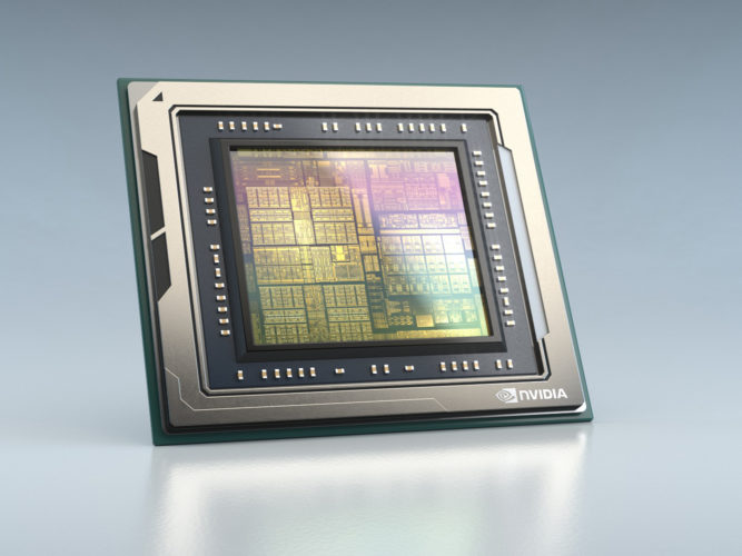
The DRIVE Orin system-on-a-chip delivers 254 trillion operations per second — ample compute headroom for a software-defined architecture. It’s designed to handle the large number of applications and deep neural networks that run simultaneously in autonomous vehicles, while achieving systematic safety standards such as ISO 26262 ASIL-D.

Equipped with the performance of DRIVE Orin, NETA vehicles will have limitless possibilities.

Aiming Higher

In addition to designing its vehicles with DRIVE Orin, NETA is working with NVIDIA technologies to develop advanced autonomous-driving capabilities.

The companies are collaborating on the design and development of a centralized cross-domain fusion computing platform for level 4 autonomy.

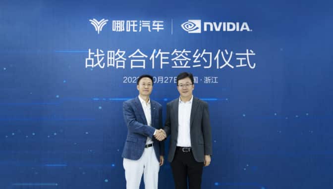
Zhang Yong, NETA Auto co-founder and CEO, with Liu Tong, NVIDIA automotive general manager in China, at the October signing ceremony.

“NETA Auto is at a new stage of development and sees technological innovation as one of the biggest enablers moving this industry forward,” said Zhang Yong, co-founder and CEO of NETA. “The close cooperation with NVIDIA will give NETA Auto a strong boost in bringing intelligent, technology-rich vehicles to market worldwide.”

The post Neural NETA: Automaker Selects NVIDIA DRIVE Orin for AI-Powered Vehicles appeared first on NVIDIA Blog.

Read More

Improve price performance of your model training using Amazon SageMaker heterogeneous clusters

This post is co-written with Chaim Rand from Mobileye.

Certain machine learning (ML) workloads, such as training computer vision models or reinforcement learning, often involve combining the GPU- or accelerator-intensive task of neural network model training with the CPU-intensive task of data preprocessing, like image augmentation. When both types of tasks run on the same instance type, the data preprocessing gets bottlenecked on CPU, leading to lower GPU utilization. This issue becomes worse with time as the throughput of newer generations of GPUs grows at a steeper pace than that of CPUs.

To address this issue, in July 2022, we launched heterogeneous clusters for Amazon SageMaker model training, which enables you to launch training jobs that use different instance types in a single job. This allows offloading parts of the data preprocessing pipeline to compute-optimized instance types, whereas the deep neural network (DNN) task continues to run on GPU or accelerated computing instance types. Our benchmarks show up to 46% price performance benefit after enabling heterogeneous clusters in a CPU-bound TensorFlow computer vision model training.

For a similar use case, Mobileye, an autonomous vehicle technologies development company, had this to share:

“By moving CPU-bound deep learning computer vision model training to run over multiple instance types (CPU and GPU/ML accelerators), using a tf.data.service based solution we’ve built, we managed to reduce time to train by 40% while reducing the cost to train by 30%. We’re excited about heterogeneous clusters allowing us to run this solution on Amazon SageMaker.”

— AI Engineering, Mobileye

In this post, we discuss the following topics:

  • How heterogeneous clusters help remove CPU bottlenecks
  • When to use heterogeneous clusters, and other alternatives
  • Reference implementations in PyTorch and TensorFlow
  • Performance benchmark results
  • Heterogeneous clusters at Mobileye

AWS’s accelerated computing instance family includes accelerators from AWS custom chips (AWS Inferentia, AWS Trainium), NVIDIA (GPUs), and Gaudi accelerators from Habana Labs (an Intel company). Note that in this post, we use the terms GPU and accelerator interchangeably.

How heterogeneous clusters remove data processing bottlenecks

Data scientists who train deep learning models aim to maximize training cost-efficiency and minimize training time. To achieve this, one basic optimization goal is to have high GPU utilization, the most expensive and scarce resource within the Amazon Elastic Compute Cloud (Amazon EC2) instance. This can be more challenging with ML workloads that combine the classic GPU-intensive neural network model’s forward and backward propagation with CPU-intensive tasks, such as data processing and augmentation in computer vision or running an environment simulation in reinforcement learning. These workloads can end up being CPU bound, where having more CPU would result in higher throughput and faster and cheaper training as existing accelerators are partially idle. In some cases, CPU bottlenecks can be solved by switching to another instance type with a higher CPU:GPU ratio. However, there are situations where switching to another instance type may not be possible due to the instance family’s architecture, storage, or networking dependencies.

In such situations, you have to increase the amount of CPU power by mixing instance types: instances with GPUs together with CPU. Summed together, this results in an overall higher CPU:GPU ratio. Until recently, SageMaker training jobs were limited to having instances of a single chosen instance type. With SageMaker heterogeneous clusters, data scientists can easily run a training job with multiple instance types, which enables offloading some of the existing CPU tasks from the GPU instances to dedicated compute-optimized CPU instances, resulting in higher GPU utilization and faster and more cost-efficient training. Moreover, with the extra CPU power, you can have preprocessing tasks that were traditionally done offline as a preliminary step to training become part of your training job. This makes it faster to iterate and experiment over both data preprocessing and DNN training assumptions and hyperparameters.

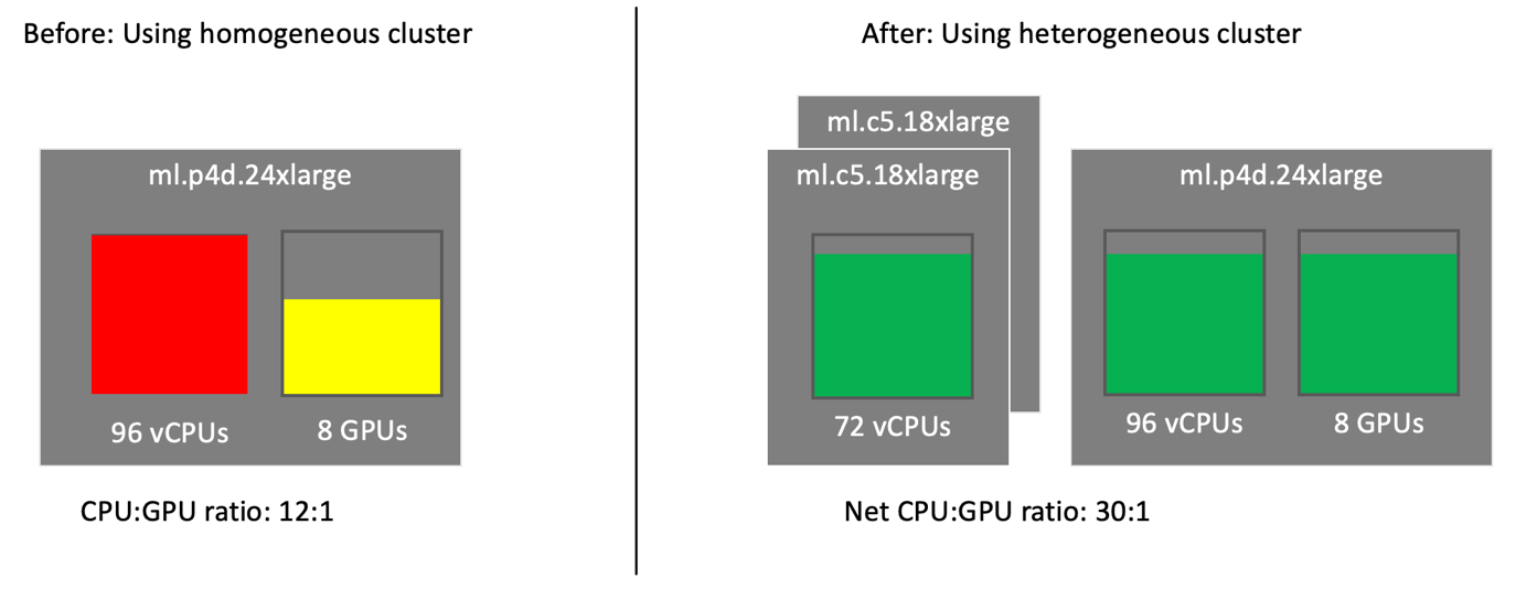
For example, consider a powerful GPU instance type, ml.p4d.24xlarge (96 vCPU, 8 x NVIDIA A100 GPUs), with a CPU:GPU ratio of 12:1. Let’s assume your training job needs 20 vCPUs to preprocess enough data to keep one GPU 100% utilized. Therefore, to keep all 8 GPUs 100% utilized, you need a 160 vCPUs instance type. However, ml.p4d.24xlarge is short of 64 vCPUs, or 40%, limiting GPU utilization to 60%, as depicted on the left of the following diagram. Would adding another ml.p4d.24xlarge instance help? No, because the job’s CPU:GPU ratio would remain the same.

With heterogeneous clusters, we can add two ml.c5.18xlarge (72 vCPU), as shown on the right of the diagram. The net total vCPU in this cluster is 210 (96+2*72), leading to a CPU:GPU ratio to 30:1. Each of these compute-optimized instances will be offloaded with a data preprocessing CPU-intensive task, and will allow efficient GPU utilization. Despite the extra cost of the ml.c5.18xlarge, the higher GPU utilization allows faster processing, and therefore higher price performance benefits.

When to use heterogeneous clusters, and other alternatives

In this section, we explain how to identify a CPU bottleneck, and discuss solving it using instance type scale up vs. heterogeneous clusters.

The quick way to identify a CPU bottleneck is to monitor CPU and GPU utilization metrics for SageMaker training jobs in Amazon CloudWatch. You can access these views from the AWS Management Console within the training job page’s instance metrics hyperlink. Pick the relevant metrics and switch from 5-minute to 1-minute resolution. Note that the scale is 100% per vCPU or GPU, so the utilization rate for an instance with 4 vCPUs/GPUs could be as high as 400%. The following figure is one such example from CloudWatch metrics, where CPU is approximately 100% utilized, indicating a CPU bottleneck, whereas GPU is underutilized.

For detailed diagnosis, run the training jobs with Amazon SageMaker Debugger to profile resource utilization status, statistics, and framework operations, by adding a profiler configuration when you construct a SageMaker estimator using the SageMaker Python SDK. After you submit the training job, review the resulting profiler report for CPU bottlenecks.

If you conclude that your job could benefit from a higher CPU:GPU compute ratio, first consider scaling up to another instance type in the same instance family, if one is available. For example, if you’re training your model on ml.g5.8xlarge (32 vCPUs, 1 GPU), consider scaling up to ml.g5.16xlarge (64 vCPUs, 1 GPU). Or, if you’re training your model using multi-GPU instance ml.g5.12xlarge (48 vCPUs, 4 GPUs), consider scaling up to ml.g5.24xlarge (96 vCPUs, 4 GPUs). Refer to the G5 instance family specification for more details.

Sometimes, scaling up isn’t an option, because there is no instance type with a higher vCPU:GPU ratio in the same instance family. For example, if you’re training the model on ml.trn1.32xlarge, ml.p4d.24xlarge, or ml.g5.48xlarge, you should consider heterogeneous clusters for SageMaker model training.

Besides scaling up, we’d like to note that there are additional alternatives to a heterogeneous cluster, like NVIDIA DALI, which offloads image preprocessing to the GPU. For more information, refer to Overcoming Data Preprocessing Bottlenecks with TensorFlow Data Service, NVIDIA DALI, and Other Methods.

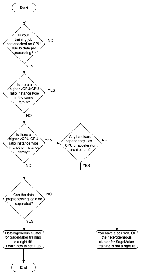
To simplify decision-making, refer to the following flowchart.

How to use SageMaker heterogeneous clusters

To get started quickly, you can directly jump to the TensorFlow or PyTorch examples provided as part of this post.

In this section, we walk you through how to use a SageMaker heterogeneous cluster with a simple example. We assume that you already know how to train a model with the SageMaker Python SDK and the Estimator class. If not, refer to Using the SageMaker Python SDK before continuing.

Prior to this feature, you initialized the training job’s Estimator class with the InstanceCount and InstanceType parameters, which implicitly assumes you only have a single instance type (a homogeneous cluster). With the release of heterogeneous clusters, we introduced the new sagemaker.instance_group.InstanceGroup class. This represents a group of one or more instances of a specific instance type, designed to carry a logical role (like data processing or neural network optimization. You can have two or more groups, and specify a custom name for each instance group, the instance type, and the number of instances for each instance group. For more information, refer to Using the SageMaker Python SDK and Using the Low-Level SageMaker APIs.

After you have defined the instance groups, you need to modify your training script to read the SageMaker training environment information that includes heterogeneous cluster configuration. The configuration contains information such as the current instance groups, the current hosts in each group, and in which group the current host resides with their ranking. You can build logic in your training script to assign the instance groups to certain training and data processing tasks. In addition, your training script needs to take care of inter-instance group communication or distributed data loading mechanisms (for example, tf.data.service in TensorFlow or generic gRPC client-server) or any other framework (for example, Apache Spark).

Let’s go through a simple example of launching a heterogeneous training job and reading the environment configuration at runtime.

  1. When defining and launching the training job, we configure two instance groups used as arguments to the SageMaker estimator:
    from sagemaker.instance_group import InstanceGroup
    data_group = InstanceGroup("data_group", "ml.c5.18xlarge", 2)
    dnn_group = InstanceGroup("dnn_group", "ml.p4d.24xlarge", 1)
    
    from sagemaker.pytorch import PyTorch
    estimator = PyTorch(...,
        entry_point='launcher.py',
        instance_groups=[data_group, dnn_group]
    )
  2. On the entry point training script (named launcher.py), we read the heterogeneous cluster configuration to whether the instance will run the preprocessing or DNN code:
    from sagemaker_training import environment
    env = environment.Environment()
    if env.current_instance_group == 'data_group': ...;

With this, let’s summarize the tasks SageMaker does on your behalf, and the tasks that you are responsible for.

SageMaker performs the following tasks:

  1. Provision different instance types according to instance group definition.
  2. Provision input channels on all or specific instance groups.
  3. Distribute training scripts and dependencies to instances.
  4. Set up an MPI cluster on a specific instance group, if defined.

You are responsible for the following tasks:

  1. Modify your start training job script to specify instance groups.
  2. Implement a distributed data pipeline (for example, tf.data.service).
  3. Modify your entry point script (see launcher.py in the example notebook) to be a single entry point that will run on all the instances, detect which instance group it’s running in, and trigger the relevant behavior (such as data processing or DNN optimization).
  4. When the training loop is over, you must make sure that your entry point process exits on all instances across all instance groups. This is important because SageMaker waits for all the instances to finish processing before it marks the job as complete and stops billing. The launcher.py script in the TensorFlow and PyTorch example notebooks provides a reference implementation of signaling data group instances to exit when DNN group instances finish their work.

Example notebooks for SageMaker heterogeneous clusters

In this section, we provide a summary of the example notebooks for both TensorFlow and PyTorch ML frameworks. In the notebooks, you can find the implementation details, walkthroughs on how the code works, code snippets that you could reuse in your training scripts, flow diagrams, and cost-comparison analysis.

Note that in both examples, you shouldn’t expect the model to converge in a meaningful way. Our intent is only to measure the data pipeline and neural network optimization throughput expressed in epoch/step time. You must benchmark with your own model and dataset to produce price performance benefits that match your workload.

Heterogeneous cluster using a tf.data.service based distributed data loader (TensorFlow)

This notebook demonstrates how to implement a heterogeneous cluster for SageMaker training using TensorFlow’s tf.data.service based distributed data pipeline. We train a deep learning computer vision model Resnet50 that requires CPU-intensive data augmentation. It uses Horvod for multi-GPU distributed data parallelism.

We run the workload in two configurations: first as a homogeneous cluster, single ml.p4d.24xlarge instance, using a standard tf.data pipeline that showcases CPU bottlenecks leading to lower GPU utilization. In the second run, we switch from a single instance type to two instance groups using a SageMaker heterogeneous cluster. This run offloads some of the data processing to additional CPU instances (using tf.data.service).

We then compare the homogeneous and heterogeneous configurations and find key price performance benefits. As shown in the following table, the heterogeneous job (86ms/step) is 2.2 times faster to train than the homogeneous job (192ms/step), making it 46% cheaper to train a model.

Example 1 (TF) ml.p4d.24xl ml.c5.18xl Price per Hour* Average Step Time Cost per Step Price Performance Improvement
Homogeneous 1 0 $37.688 192 ms $0.201 .
Heterogeneous 1 2 $45.032 86 ms $0.108 46%

* Price per hour is based on us-east-1 SageMaker on-demand pricing

This speedup is made possible by utilizing the extra vCPU, provided by the data group, and faster preprocessing. See the notebook for more details and graphs.

Heterogeneous cluster using a gRPC client-server based distributed data loader (PyTorch)

This notebook demonstrates a sample workload using a heterogeneous cluster for SageMaker training using a gRPC client-server based distributed data loader. This example uses a single GPU. We use the PyTorch model based on the following official MNIST example. The training code has been modified to be heavy on data preprocessing. We train this model in both homogeneous and heterogeneous cluster modes, and compare price performance.

In this example, we assumed the workload can’t benefit from multiple GPUs, and has dependency on a specific GPU architecture (NVIDIA V100). We ran both homogeneous and heterogeneous training jobs, and found key price performance benefits, as shown in the following table. The heterogeneous job (1.19s/step) is 6.5 times faster to train than the homogeneous job (0.18s/step), making it 77% cheaper to train a model.

Example 2 (PT) ml.p3.2xl ml.c5.9xl Price per Hour* Average Step Time Cost per Step Price Performance Improvement
Homogeneous 1 0 $3.825 1193 ms $0.127 .
Heterogeneous 1 1 $5.661 184 ms $0.029 77%

* Price per hour is based on us-east-1 SageMaker on-demand pricing

This is possible because with a higher CPU count, we could use 32 data loader workers (compared to 8 with ml.p3.2xlarge) to preprocess the data and kept GPU close to 100% utilized at frequent intervals. See the notebook for more details and graphs.

Heterogeneous clusters at Mobileye

Mobileye, an Intel company, develops Advanced Driver Assistance Systems (ADAS) and autonomous vehicle technologies with the goal of revolutionizing the transportation industry, making roads safer, and saving lives. These technologies are enabled using sophisticated computer vision (CV) models that are trained using SageMaker on large amounts of data stored in Amazon Simple Storage Service (Amazon S3). These models use state-of-the-art deep learning neural network techniques.

We noticed that for one of our CV models, the CPU bottleneck was primarily caused by heavy data preprocessing leading to underutilized GPUs. For this specific workload, we started looking at alternative solutions, evaluated distributed data pipeline technologies with heterogeneous clusters based on EC2 instances, and came up with reference implementations for both TensorFlow and PyTorch. The release of the SageMaker heterogeneous cluster allows us to run this and similar workloads on SageMaker to achieve improved price performance benefits.

Considerations

With the launch of the heterogeneous cluster feature, SageMaker offers a lot more flexibility in mixing and matching instance types within your training job. However, consider the following when using this feature:

  • The heterogeneous cluster feature is available through SageMaker PyTorch and TensorFlow framework estimator classes. Supported frameworks are PyTorch v1.10 or later and TensorFlow v2.6 or later.
  • All instance groups share the same Docker image.
  • All instance groups share the same training script. Therefore, your training script should be modified to detect which instance group it belongs to and fork runs accordingly.
  • The training instances hostnames (for example, alog-1, algo-2, and so on) are randomly assigned, and don’t indicate which instance group they belong to. To get the instance’s role, we recommend getting its instance group membership during runtime. This is also relevant when reviewing logs in CloudWatch, because the log stream name [training-job-name]/algo-[instance-number-in-cluster]-[epoch_timestamp] has the hostname.
  • A distributed training strategy (usually an MPI cluster) can be applied only to one instance group.
  • SageMaker Managed Warm Pools and SageMaker Local Mode cannot currently be used with heterogeneous cluster training.

Conclusion

In this post, we discussed when and how to use the heterogeneous cluster feature of SageMaker training. We demonstrated a 46% price performance improvement on a real-world use case and helped you get started quickly with distributed data loader (tf.data.service and gRPC client-server) implementations. You can use these implementations with minimal code changes in your existing training scripts.

To get started, try out our example notebooks. To learn more about this feature, refer to Train Using a Heterogeneous Cluster.


About the authors

Gili Nachum is a senior AI/ML Specialist Solutions Architect who works as part of the EMEA Amazon Machine Learning team. Gili is passionate about the challenges of training deep learning models, and how machine learning is changing the world as we know it. In his spare time, Gili enjoy playing table tennis.

Hrushikesh Gangur is a principal solutions architect for AI/ML startups with expertise in both ML Training and AWS Networking. He helps startups in Autonomous Vehicle, Robotics, CV, NLP, MLOps, ML Platform, and Robotics Process Automation technologies to run their business efficiently and effectively on AWS. Prior to joining AWS, Hrushikesh acquired 20+ years of industry experience primarily around Cloud and Data platforms.

Gal Oshri is a Senior Product Manager on the Amazon SageMaker team. He has 7 years of experience working on Machine Learning tools, frameworks, and services.

Chaim Rand is a machine learning algorithm developer working on deep learning and computer vision technologies for Autonomous Vehicle solutions at Mobileye, an Intel Company. Check out his blogs.

Read More

Reduce food waste to improve sustainability and financial results in retail with Amazon Forecast

With environmental, social, and governance (ESG) initiatives becoming more important for companies, our customer, one of Greater China region’s top convenience store chains, has been seeking a solution to reduce food waste (currently over $3.5 million USD per year). Doing so will allow them to not only realize substantial operating savings, but also support corporate sustainability goals.

In this post, we focus on forecasting demand of freshly prepared food by retail convenience stores. Our customer sells ready-to-eat food items with a short shelf life—typically 2–3 days. They faced two challenges: how to reduce food waste, and how to manage forecast models for over 10,000 SKUs and thousands of stores efficiently and at scale.

With Amazon Forecast, and support from the AWS ProServe team and AWS Machine Learning Solutions Lab, our customer—with limited internal data scientists—now has state-of-the-art forecasting capabilities. Within a few months, this forecasting solution has helped them reduce product waste by 37%, resulting in cost savings of 22% across 168 stores and three merchandise categories.

To achieve these operational benefits, they implemented a number of best practice processes, including a fast data iteration and testing cycle, and parallel testing to find optimal data combinations. They also established data processing and forecasting pipelines, which can scale to thousands of stores and product categories, and developed a scalable reference architecture to be used for future extensions.

The fresh foods ESG challenge

In addition to selling environmentally sustainable products, it’s also important for the retail industry to strive for environmentally friendly processes that minimize waste. Advanced inventory forecasting using machine learning (ML) allows retail stores to maximize sales and minimize waste through more effective inventory management and turnover. Inventory that can’t be sold is a problem for convenience store chains—it drives financial losses and furthers negative environmental effects through excess usage of energy inputs and inefficient production processes. And due to large volumes, short-dated fresh food items can play a big role in both financial and sustainability results.

Besides having a short shelf life, additional demand forecasting challenges for fresh food include rapid turnover, frequent new product launches, and high SKU volumes. Specifically:

  • Compared to other categories, short-dated perishables must be sold within a short time window, otherwise they will expire and be discarded. Therefore, accurate forecasting is more important than for items that can be stored and sold over a longer time period.
  • New product launches are frequent, making forecasting more challenging at the SKU-level (the cold start problem).
  • A large number of items can cause model management issues for traditional algorithms such as ARIMA, which are configured for each item. Many models will need to be maintained, which is both costly and hard to scale.

Inventory forecasting

Amazon Forecast is a fully managed AI/ML service from AWS, and includes both statistical and deep learning algorithms that are based on over 20 years of forecasting experience. With item-level ensemble modeling and automatic model hyperparameter optimization, it provides forecasts that are up to 40% more accurate that using traditional methods alone. In addition, features such as predictor retraining can reduce training time and cost by up to 50%.

To optimize inventory forecasting, we looked at the main drivers of demand. Even within the fresh food category, there are items that are more popular—with higher inventory turnover—and items that sell slower. By separating popular from unpopular items and training predictors, we found that predictors can fit the dataset better and enhance model accuracy with different statistical distributions. In addition, because Forecast provides probabilistic forecasts based on customer-selected quantiles, we set up prediction quantiles based on item expiration dates and item profitability.

To implement demand forecasting that enhances sustainability, we also considered industry-specific properties:

  • Short lead times
  • High order frequencies
  • Product alternatives and substitutes
  • Consumer psychology (often, consumers are more likely to make a purchase if they have a diverse set of products to select from)

To balance shelf diversity against inventory wastage, we not only produced daily demand forecasts, but also performed what-if analyses to optimize promotion of unsold items before they expire.

We were able to incorporate these considerations and address our customer’s requirements with Forecast. In the next section, we walk through how the customer solution has been created in more detail.

Solution overview

To train a predictor, training data is ingested into data storage from a data source, using one of the formats supported by Forecast. Amazon Simple Storage Service (Amazon S3) is an object storage service offering industry-leading scalability, data availability, security, and performance. In the ingestion phase, we transform data from our source to the Forecast dataset format. Forecast uses three types of data: target time series (TTS), which is required, and related time series (RTS) and item metadata (IM), both of which are optional.

We started with the most-wasted SKUs at the stores that had the most waste. To forecast each store’s daily demand, we first started with time series (revenues, inventories, promotions) and then fine-tuned our approach based on store properties such as whether it’s a franchise or company-owned store, store type, restroom availability, store size (small or large), and store age. We also used industry knowledge, such as local holidays, promotions, weather, and daily traffic. Our TTS dataset consisted of timestamp, item ID, and demand; RTS consisted of timestamp, item ID, discount, inventory, and weather; and the IM dataset consisted of item ID, category, and store infrastructures. To quantify the importance of these features on our forecasts, we used explainability—a Forecast built-in feature that measures the relative impact of different attributes on forecast values.

A dataset must be created and associated with a dataset group to train the predictor. When creating a predictor, Forecast automatically selects the right algorithms, tunes hyperparameters, and performs ensemble modeling. In an interesting finding from this case, we used cross-COVID-19 data (from 2018–2021) to train the model and found that we didn’t need to add other COVID-19 features such as number of daily confirmed cases. The deep neural network models can learn directly from daily revenue.

The following diagram illustrates the solution architecture.

Inventory forecasting solution architecture

Our customer maintains their transactional records in Amazon Relational Database Service (Amazon RDS). We also use AWS Glue to conduct ETL (extract, transform, and load), read data covering the target SKUs across a meaningful time range, and load data to Amazon S3 with an indicated prefix. After data is loaded to Amazon S3, an S3 event triggers AWS Lambda and invokes AWS Step Functions as an orchestration tool.

In Step Functions, we prepare datasets that include target time series, related time series, and item metadata. We use an AWS Glue job to process the data into an S3 bucket. We can then call a Forecast API to create a dataset group and import data from the processed S3 bucket. When those datasets are ready, we can start to train the predictor.

To train a predictor, Forecast ensemble models six different algorithms and applies the optimal combination of algorithms to each time series in your dataset. We use the AutoPredictor API, which is also accessible through the Forecast console.

After the predictors have been created, we evaluated their quality metrics in the predictors dashboard. You can choose the predictor name to examine detailed results such as Weighted Quantile Loss (wQL), Weighted Absolute Percentage Error (WAPE), Mean Absolute Scaled Error (MASE), Root Mean Squared Error (RMSE), and Mean Absolute Percentage Error (MAPE). For customized evaluation and analysis, you can also export the forecasted values to evaluate predictor quality metrics. In this case, we used the customer’s original metric—MAPE—to produce a side-by-side comparison with the customer’s legacy model (ARIMA), and ensure that the Forecast model produced better results (a lower MAPE). For future model quality analyses, we recommended that the customer use RMSE, which better accounts for the fact that different items have different sales volumes.

After our predictor was ready, we generated forecast results for every item (item_id) and dimension (store_id) indicated in our target time series dataset. Forecast places results in an S3 bucket with the S3 prefix as the destination.

Forecast results are generated in the S3 bucket, triggering a Lambda function and writing the forecast result to Amazon Aurora for the end-user to query. To provide the forecasting result to the client side, we use Amazon API Gateway as the entry point and query Aurora through the Lambda function.

To automate this process, we used Step Functions, and we also maintain an Amazon SageMaker notebook for data scientists to featurize and test different data variations in the training dataset to find optimal data combinations.

Summary and next steps

In this post, we showed how to use Forecast to minimize waste through more effective inventory forecasting of food products with a short shelf life. The application of ML-based forecasting helped our retail customer reduce product waste by 37% and costs by 22% across 168 stores and three merchandise categories. Moreover, the reference architecture is able to support scaling to thousands of stores and product categories. These efforts not only improved financial outcomes, but also demonstrated their commitment to more sustainable, enviornmental friendly food practices. Together, these achievements helped our customer progress toward their ESG initiatives.

Next up for the team is using the what-if analysis capabilities of Forecast to further test the impact on demand, add subcategories for daily demand forecasting, and scale to more stores. In addition, the team will keep iterating the model to continue reducing food waste, and optimize processes to deliver more sustainable and environmentally friendly results.

To use Forecast to improve retail demand forecasting and support better environmental outcomes, you can access the service through the AWS Management Console, or through our AWS CloudFormation-based solution guidance on GitHub. To learn more about how to use Forecast, check out Amazon Forecast resources.


About the Authors

auth-JosieJosie Cheng is a HKT AI/ML Go-To-Market at AWS. Her current focus is on business transformation in retail and CPG through data and ML to fuel tremendous enterprise growth. Before joining AWS, Josie worked for Amazon Retail and other China and US internet companies as a Growth Product Manager.

Ray Wang is a Solutions Architect at AWS. With 8 years of experience in the IT industry, Ray is dedicated to building modern solutions on the cloud, especially in NoSQL, big data, and machine learning. As a hungry go-getter, he passed all 12 AWS certificates to make his technical field not only deep but wide. He loves to read and watch sci-fi movies in his spare time.

Shanger Lin is Data Scientist and Consultant at AWS, leveraging machine learning, cloud computing, and data strategy to enable customers with digital transformation and to extract impact from data.

Dan Sinnreich is a Sr. Product Manager for Amazon Forecast. His focus is helping companies drive better business decisions with ML-based forecasting. Outside of work, he can be found playing hockey, reading science fiction, and scuba diving.

Read More

Microsoft Experience Centers Display Scalable, Real-Time Graphics With NVIDIA RTX and Mosaic Technology

When customers walk into a Microsoft Experience Center in New York City, Sydney or London, they’re instantly met with stunning graphics displayed on multiple screens and high-definition video walls inside a multi-story building.

Built to showcase the latest technologies, Microsoft Experience Centers surround customers with vibrant, immersive graphics as they explore new products, watch technical demos, get hands-on experience with the latest solutions and learn more about Microsoft.

To create these engaging visual experiences in real time and on a scalable level, Microsoft sought a solution that would allow it to power high-quality graphics spanning large multi-display walls — without any gaps, artifacts or misalignment in the visuals.

It was also important that the software allowed for simplicity when managing and monitoring the display environments. Microsoft chose NVIDIA RTX A6000 GPUs, along with NVIDIA Mosaic and Quadro Sync technology, which provided support for the demanding visualizations across displays and enabled viewers to see everything as one unified visual.

All images courtesy of Microsoft.

Putting High-Quality Graphics on Full Display

The display walls in Microsoft Experience Centers feature many detailed visuals and scenes that require powerful graphics-computing performance. The HD walls display changing, detailed renders of various Microsoft products. These graphics are created with custom camera angles and fly-throughs.

Once the visuals were created, the team had to synchronize the graphics and ensure the systems were appearing in unison. In each Microsoft Experience Center, the team uses a visualization cluster of up to six systems, with a pair of RTX A6000 GPUs in each. Unreal Engine with nDisplay technology was used to make the Microsoft Video Player work in a cluster setting.

“NVIDIA RTX A6000 GPUs provide the smooth and powerful performance that is required to run high-quality visuals across a large number of displays,” said Chris Haklitch, principal PM lead at Microsoft. “The enterprise reliability and support NVIDIA provides, along with the software and hardware only available with professional RTX GPUs, helped make our vision possible.”

With NVIDIA Mosaic multi-display technology, Microsoft can treat multiple displays as a single desktop, without application software changes or visual artifacts. This enabled the walls of HD displays to be shown as a single unified visual.

NVIDIA Quadro Sync II is a key technology that enables all displays to appear as a single continuous image. Designed for flexibility and scalability, Quadro Sync helps connect and synchronize the NVIDIA RTX GPUs to its attached displays.

Microsoft also used an NVIDIA Enterprise Management Toolkit called NVWMI, which lets IT administrators create scripts and programs for many administrative tasks and functions. With NVWMI, Microsoft can remotely monitor the GPU-powered display environments, ensuring simple access to adjust display settings. Microsoft also used NVWMI to monitor the GPU thermals and performance to meet the demands of ongoing store operation.

NVIDIA Mosaic, Quadro Sync and NVWMI are professional software features that are only available with NVIDIA RTX professional GPUs.

Learn more about NVIDIA RTX professional solutions for deploying scalable visualizations.

The post Microsoft Experience Centers Display Scalable, Real-Time Graphics With NVIDIA RTX and Mosaic Technology appeared first on NVIDIA Blog.

Read More

Research Focus: Week of October 24, 2022

Research Focus - October 2022

Welcome to Research Focus, a new series of blog posts that highlights notable publications, events, code/datasets, new hires and other milestones from across the research community at Microsoft.

Meet the 2022 recipients of the Microsoft Research Global PhD Fellowship

Microsoft is thrilled to announce the 2022 Microsoft Research Global PhD Fellows from around the world. The program aims to empower the next generation of computing-related research talent. Microsoft recognizes the value of diversity in computing and aims to increase the pipeline of talent receiving advanced degrees in computing-related fields to build a stronger and inclusive computing-related research community. We currently offer PhD fellowships in Asia-Pacific, Canada and the United States, EMEA (Europe, Middle East, Africa), Latin America, Australia and New Zealand.


Making the most of text semantics to improve biomedical vision-language processing 

Benedikt Boecking, Naoto Usuyama, Shruthi Bannur, Daniel Coelho de Castro, Anton Schwaighofer, Stephanie Hyland, Maria Teodora Wetscherek, Tristan Naumann, Aditya Nori, Javier Alvarez-Valle, Hoifung Poon, Ozan Oktay

Multi-modal data abounds in biomedicine, such as radiology images and reports. Interpreting this data at scale is essential for improving clinical care workflows and accelerating clinical research. With its complex semantics, biomedical text poses additional challenges in vision-language modelling, and previous work has used insufficiently adapted models that lack domain-specific language understanding. In this study, we show that principled textual semantic modelling can substantially improve contrastive learning in biomedical vision-language processing (VLP). We release a language model (CXR-BERT) that achieves state-of-the-art results in radiology natural language inference through its improved vocabulary and novel language pretraining objective. Furthermore, we propose a self-supervised joint VLP approach (BioViL) with a focus on better text modelling. It establishes new state-of-the-art results on a wide range of publicly available benchmarks, in part by leveraging our novel domain-specific language model. As part of this study, a new dataset (MS-CXR) is released to facilitate the study of complex semantic modelling in biomedical VLP, which includes locally aligned phrase grounding annotations by radiologists. A broad evaluation, including on this new dataset, shows that our contrastive learning approach outperforms prior methods in segmentation tasks, despite only using a global-alignment objective.


Spotlight: On-Demand EVENT

Microsoft Research Summit 2022

On-Demand
Watch now to learn about some of the most pressing questions facing our research community and listen in on conversations with 120+ researchers around how to ensure new technologies have the broadest possible benefit for humanity.

How AI Happens podcast: A conversation with AI4Science Senior Director Bonnie Kruft

Microsoft’s AI4Science Senior Director Bonnie Kruft was interviewed for a recent podcast in the “How AI Happens” series. Tune in to learn about her journey from earning a Ph.D. focused on quantum chemistry to working in AI and machine learning. She explains how she first discovered her love of data science, and how her Ph.D. equipped her with the skills she needed to succeed. The conversation also covers the data science approach to problem-solving, deep learning emulators and the impact that machine learning could have on the natural sciences.


Recent researcher awards and accomplishments

Ronen Eldan wins prestigious New Horizons in Mathematics Prize

Ronen Eldan, of Microsoft Research and the Weizmann Institute of Science, was awarded the prestigious New Horizons in Mathematics Prize by The Breakthrough Prize Foundation. Eldan was recognized for creating the stochastic localization method, which has led to significant progress in several open problems in high-dimensional geometry and probability, including Jean Bourgain’s slicing problem and the KLS conjecture. 

The Breakthrough Prize Foundation and its founding sponsors – Sergey Brin, Priscilla Chan and Mark Zuckerberg, Julia and Yuri Milner, and Anne Wojcicki – announced the 2023 award winners in September. The foundation highlights game-changing discoveries in fundamental physics, life sciences and mathematics, along with early-career scientists who have made significant contributions to their fields.

Gary J. Sullivan named Fellow of the Society of Motion Picture and Television Engineers

 Microsoft’s Gary J. Sullivan was recognized as a 2022 Fellow of the Society of Motion Picture and Television Engineers (SMPTE). The membership grade of fellow is awarded to individuals who have, by proficiency and contributions, attained an outstanding rank among engineers or executives in the motion-picture, television or related industries, according to SMPTE. 

Sullivan is a principal video and image technology standardization program manager at Microsoft Research in Redmond, Washington. At Microsoft, he has been the originator and lead designer of the DirectX Video Acceleration (DXVA) video decoding feature of Microsoft Windows and in the international standardization community, he has led team projects that have been recognized by three Emmy Awards. His standardization work includes chairing or co-chairing various projects related to media compression in the JPEG, MPEG, and VCEG standards groups, including the AVC (H.264), HEVC (H.265) and VVC (H.266) video compression codec design projects. He is currently the chair of ISO/IEC JTC 1/SC 29, which oversees the work of JPEG and MPEG, and the Rapporteur of video and image coding in ITU-T SG16. 

The post Research Focus: Week of October 24, 2022 appeared first on Microsoft Research.

Read More

Make Gaming a Priority: Special Membership Discount Hits GeForce NOW for Limited Time

This spook-tacular Halloween edition of GFN Thursday features a special treat: 40% off a six-month GeForce NOW Priority Membership — get it for just $29.99 for a limited time.

Several sweet new games are also joining the GeForce NOW library.

Creatures of the night can now stream vampire survival game V Rising from the cloud. The fang-tastic fun arrives just in time to get started with the game’s “Bloodfeast” Halloween event and free weekend.

It leads the pack for 12 total games streaming this week, including new releases like Victoria 3.

Elevate Your Gaming to Priority

Through Sunday, Nov. 20, upgrade to a six-month Priority Membership for just $29.99, 40% off the standard price of $49.99.

Priority Membership Sale
Don’t miss out on this special offer.

Power up devices compatible with GeForce NOW for the boost of a full gaming rig in the cloud. Get faster access to games with priority access to gaming servers. Enjoy extended play times with six-hour gaming sessions. And take supported games to the next level with beautifully ray-traced graphics with RTX ON.

This limited-time offer is valid for new users and existing ones upgrading from a free or one-month Priority Membership, as well as for those who are on an active promotion or gift card.

Check out the GeForce NOW membership page for more information on Priority benefits.

Sink Your Teeth Into ‘V Rising’

Awaken as a vampire after centuries of slumber and survive in a vast world teeming with mythical horrors and danger streaming V Rising on GeForce NOW.

Raise a castle, gather valuable resources and weapons, develop dark powers and convert humans into loyal servants in the quest to raise a vampire empire. Make allies or enemies online, or play solo in the game of blood, power and betrayal.

The game arrives just in time for members to join in on the Bloodfeast, where all creatures of the night are invited to play for free from Oct. 28-Nov. 1. V Rising players will be able to claim the free “Halloween Haunted Nights Castle DLC Pack” through Monday, Nov. 7.

Rule the night playing V Rising across your devices, even on a mobile phone. RTX 3080 members can even stream at 4K resolution on the PC and Mac apps.

Something Wicked Awesome This Way Comes

Gamers can get right into the frightful fun by checking out the horror and thriller titles included in the Halloween games row in the GeForce NOW app.

If games with a bit of a bite aren’t your thing, that’s okay. There’s something for everyone on the cloud.

Victoria 3 on GeForce NOW
This one’s for the history books. Balance competing interests to build an ideal society in the transformative 19th century.

Look out for the 12 total games available to stream today, including 3 new releases like Victoria 3.

  • Victoria 3 (New release on Steam)
  • Star Ocean: The Divine Force (New release on Steam, Oct. 27)
  • Paper Cut Mansion (New release on Steam and Epic Games, Oct. 27)
  • Saturnalia (New release on Epic Games, Oct. 27)
  • Asterigos: Curse of the Stars (Epic Games)
  • Draw Slasher (Steam)
  • Five Nights at Freddy’s: Security Breach (Steam and Epic Games)
  • Guild Wars: Game of the Year (Steam)
  • Labyrinthine (Steam)
  • Sniper Elite 5 (Steam)
  • Volcanoids (Steam)
  • V Rising (Steam)

Also, try the new LEGO Bricktales demo before buying the full game on Steam.

Additionally, Guild Wars Trilogy, announced previously, will not be coming to the cloud.

Ready for the scary season? There’s only one question left. Let us know your choice on Twitter or in the comments below.

The post Make Gaming a Priority: Special Membership Discount Hits GeForce NOW for Limited Time appeared first on NVIDIA Blog.

Read More

3 Questions: How AI image generators could help robots

3 Questions: How AI image generators could help robots

AI image generators, which create fantastical sights at the intersection of dreams and reality, bubble up on every corner of the web. Their entertainment value is demonstrated by an ever-expanding treasure trove of whimsical and random images serving as indirect portals to the brains of human designers. A simple text prompt yields a nearly instantaneous image, satisfying our primitive brains, which are hardwired for instant gratification. 

Although seemingly nascent, the field of AI-generated art can be traced back as far as the 1960s with early attempts using symbolic rule-based approaches to make technical images. While the progression of models that untangle and parse words has gained increasing sophistication, the explosion of generative art has sparked debate around copyright, disinformation, and biases, all mired in hype and controversy. Yilun Du, a PhD student in the Department of Electrical Engineering and Computer Science and affiliate of MIT’s Computer Science and Artificial Intelligence Laboratory (CSAIL), recently developed a new method that makes models like DALL-E 2 more creative and have better scene understanding. Here, Du describes how these models work, whether this technical infrastructure can be applied to other domains, and how we draw the line between AI and human creativity. 

Q: AI-generated images use something called “stable diffusion” models to turn words into astounding images in just a few moments. But for every image used, there’s usually a human behind it. So what’s the the line between AI and human creativity? How do these models really work? 

A: Imagine all of the images you could get on Google Search and their associated patterns. This is the diet these models are fed on. They’re trained on all of these images and their captions to generate images similar to the billions of images it has seen on the internet.

Let’s say a model has seen a lot of dog photos. It’s trained so that when it gets a similar text input prompt like “dog,” it’s able to generate a photo that looks very similar to the many dog pictures already seen. Now, more methodologically, how this all works dates back to a very old class of models called “energy-based models,” originating in the ’70’s or ’80’s.

In energy-based models, an energy landscape over images is constructed, which is used to simulate the physical dissipation to generate images. When you drop a dot of ink into water and it dissipates, for example, at the end, you just get this uniform texture. But if you try to reverse this process of dissipation, you gradually get the original ink dot in the water again. Or let’s say you have this very intricate block tower, and if you hit it with a ball, it collapses into a pile of blocks. This pile of blocks is then very disordered, and there’s not really much structure to it. To resuscitate the tower, you can try to reverse this folding process to generate your original pile of blocks.

The way these generative models generate images is in a very similar manner, where, initially, you have this really nice image, where you start from this random noise, and you basically learn how to simulate the process of how to reverse this process of going from noise back to your original image, where you try to iteratively refine this image to make it more and more realistic. 

In terms of what’s the line between AI and human creativity, you can say that these models are really trained on the creativity of people. The internet has all types of paintings and images that people have already created in the past. These models are trained to recapitulate and generate the images that have been on the internet. As a result, these models are more like crystallizations of what people have spent creativity on for hundreds of years. 

At the same time, because these models are trained on what humans have designed, they can generate very similar pieces of art to what humans have done in the past. They can find patterns in art that people have made, but it’s much harder for these models to actually generate creative photos on their own. 

If you try to enter a prompt like “abstract art” or “unique art” or the like, it doesn’t really understand the creativity aspect of human art. The models are, rather, recapitulating what people have done in the past, so to speak, as opposed to generating fundamentally new and creative art.

Since these models are trained on vast swaths of images from the internet, a lot of these images are likely copyrighted. You don’t exactly know what the model is retrieving when it’s generating new images, so there’s a big question of how you can even determine if the model is using copyrighted images. If the model depends, in some sense, on some copyrighted images, are then those new images copyrighted? That’s another question to address. 

Q: Do you believe images generated by diffusion models encode some sort of understanding about natural or physical worlds, either dynamically or geometrically? Are there efforts toward “teaching” image generators the basics of the universe that babies learn so early on? 

A: Do they understand, in code, some grasp of natural and physical worlds? I think definitely. If you ask a model to generate a stable configuration of blocks, it definitely generates a block configuration that’s stable. If you tell it, generate an unstable configuration of blocks, it does look very unstable. Or if you say “a tree next to a lake,” it’s roughly able to generate that. 

In a sense, it seems like these models have captured a large aspect of common sense. But the issue that makes us, still, very far away from truly understanding the natural and physical world is that when you try to generate infrequent combinations of words that you or I in our working our minds can very easily imagine, these models cannot.

For example, if you say, “put a fork on top of a plate,” that happens all the time. If you ask the model to generate this, it easily can. If you say, “put a plate on top of a fork,” again, it’s very easy for us to imagine what this would look like. But if you put this into any of these large models, you’ll never get a plate on top of a fork. You instead get a fork on top of a plate, since the models are learning to recapitulate all the images it’s been trained on. It can’t really generalize that well to combinations of words it hasn’t seen. 

A fairly well-known example is an astronaut riding a horse, which the model can do with ease. But if you say a horse riding an astronaut, it still generates a person riding a horse. It seems like these models are capturing a lot of correlations in the datasets they’re trained on, but they’re not actually capturing the underlying causal mechanisms of the world.

Another example that’s commonly used is if you get very complicated text descriptions like one object to the right of another one, the third object in the front, and a third or fourth one flying. It really is only able to satisfy maybe one or two of the objects. This could be partially because of the training data, as it’s rare to have very complicated captions But it could also suggest that these models aren’t very structured. You can imagine that if you get very complicated natural language prompts, there’s no manner in which the model can accurately represent all the component details.

Q: You recently came up with a new method that uses multiple models to create more complex images with better understanding for generative art. Are there potential applications of this framework outside of image or text domains? 

A: We were really inspired by one of the limitations of these models. When you give these models very complicated scene descriptions, they aren’t actually able to correctly generate images that match them. 

One thought is, since it’s a single model with a fixed computational graph, meaning you can only use a fixed amount of computation to generate an image, if you get an extremely complicated prompt, there’s no way you can use more computational power to generate that image.

If I gave a human a description of a scene that was, say, 100 lines long versus a scene that’s one line long, a human artist can spend much longer on the former. These models don’t really have the sensibility to do this. We propose, then, that given very complicated prompts, you can actually compose many different independent models together and have each individual model represent a portion of the scene you want to describe.

We find that this enables our model to generate more complicated scenes, or those that more accurately generate different aspects of the scene together. In addition, this approach can be generally applied across a variety of different domains. While image generation is likely the most currently successful application, generative models have actually been seeing all types of applications in a variety of domains. You can use them to generate different diverse robot behaviors, synthesize 3D shapes, enable better scene understanding, or design new materials. You could potentially compose multiple desired factors to generate the exact material you need for a particular application.

One thing we’ve been very interested in is robotics. In the same way that you can generate different images, you can also generate different robot trajectories (the path and schedule), and by composing different models together, you are able to generate trajectories with different combinations of skills. If I have natural language specifications of jumping versus avoiding an obstacle, you could also compose these models together, and then generate robot trajectories that can both jump and avoid an obstacle . 

In a similar manner, if we want to design proteins, we can specify different functions or aspects — in an analogous manner to how we use language to specify the content of the images — with language-like descriptions, such as the type or functionality of the protein. We could then compose these together to generate new proteins that can potentially satisfy all of these given functions. 

We’ve also explored using diffusion models on 3D shape generation, where you can use this approach to generate and design 3D assets. Normally, 3D asset design is a very complicated and laborious process. By composing different models together, it becomes much easier to generate shapes such as, “I want a 3D shape with four legs, with this style and height,” potentially automating portions of 3D asset design. 

Read More