NVIDIA Breaks 16 AI Performance Records in Latest MLPerf Benchmarks

NVIDIA Breaks 16 AI Performance Records in Latest MLPerf Benchmarks

NVIDIA delivers the world’s fastest AI training performance among commercially available products, according to MLPerf benchmarks released today.

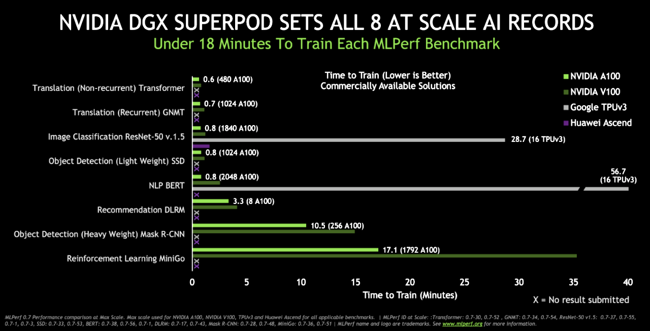
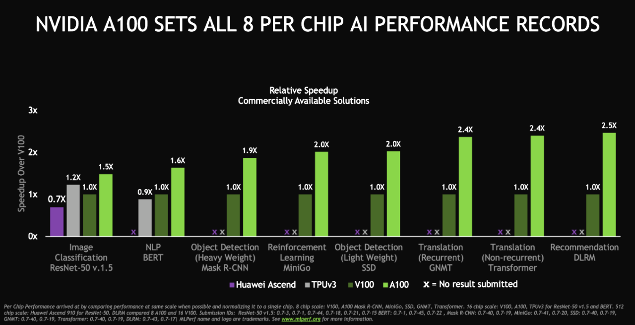
The A100 Tensor Core GPU demonstrated the fastest performance per accelerator on all eight MLPerf benchmarks. For overall fastest time to solution at scale, the DGX SuperPOD system, a massive cluster of DGX A100 systems connected with HDR InfiniBand, also set eight new performance milestones. The real winners are customers applying this performance today to transform their businesses faster and more cost effectively with AI.

This is the third consecutive and strongest showing for NVIDIA in training tests from MLPerf, an industry benchmarking group formed in May 2018. NVIDIA set six records in the first MLPerf training benchmarks in December 2018 and eight in July 2019.

NVIDIA set records in the category customers care about moshttps://mlperf.org/t: commercially available products. We ran tests using our latest NVIDIA Ampere architecture as well as our Volta architecture.

The NVIDIA DGX SuperPOD system set new milestones for AI training at scale.

NVIDIA was the only company to field commercially available products for all the tests. Most other submissions used the preview category for products that may not be available for several months or the research category for products not expected to be available for some time.

NVIDIA Ampere Ramps Up in Record Time

In addition to breaking performance records, the A100, the first processor based on the NVIDIA Ampere architecture, hit the market faster than any previous NVIDIA GPU. At launch, it powered NVIDIA’s third-generation DGX systems, and it became publicly available in a Google cloud service just six weeks later.

Also helping meet the strong demand for A100 are the world’s leading cloud providers, such as Amazon Web Services, Baidu Cloud, Microsoft Azure and Tencent Cloud, as well as dozens of major server makers, including Dell Technologies, Hewlett Packard Enterprise, Inspur and Supermicro.

Users across the globe are applying the A100 to tackle the most complex challenges in AI, data science and scientific computing.

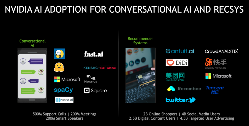
Some are enabling a new wave of recommendation systems or conversational AI applications while others power the quest for treatments for COVID-19. All are enjoying the greatest generational performance leap in eight generations of NVIDIA GPUs.

The NVIDIA Ampere architecture swept all eight tests of commercially available accelerators.

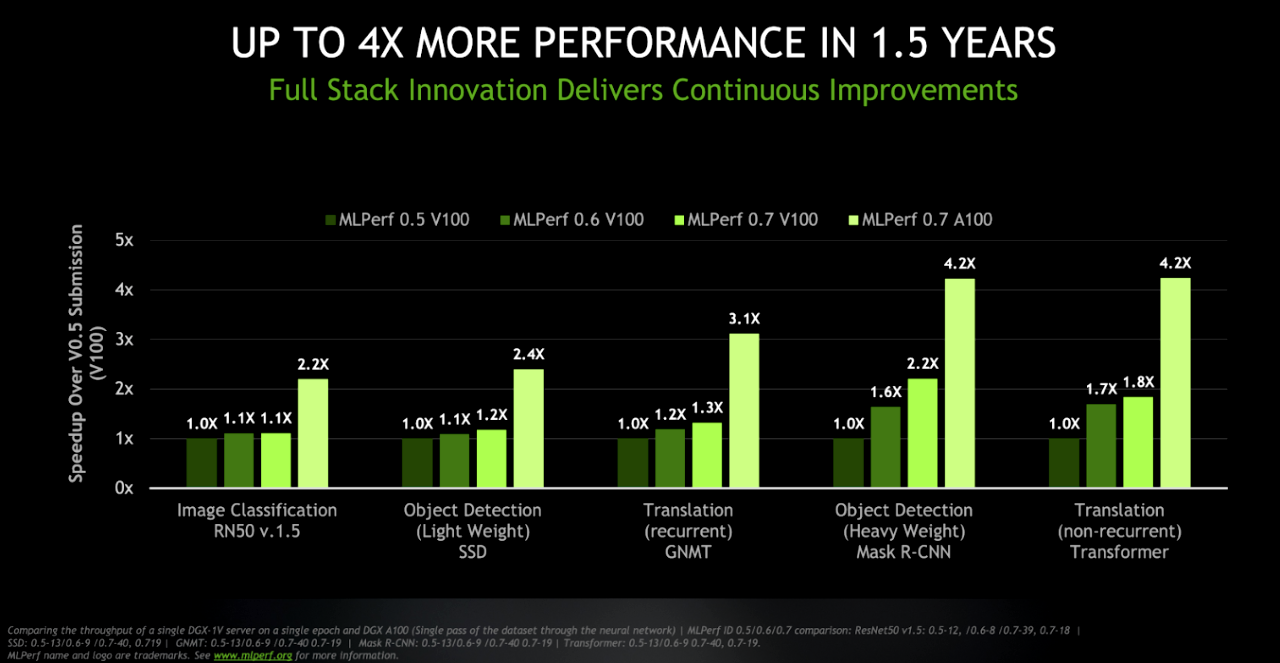
A 4x Performance Gain in 1.5 Years

The latest results demonstrate NVIDIA’s focus on continuously evolving an AI platform that spans processors, networking, software and systems.

For example, the tests show at equivalent throughput rates today’s DGX A100 system delivers up to 4x the performance of the system that used V100 GPUs in the first round of MLPerf training tests. Meanwhile, the original DGX-1 system based on NVIDIA V100 can now deliver up to 2x higher performance thanks to the latest software optimizations.

These gains came in less than two years from innovations across the AI platform. Today’s NVIDIA A100 GPUs — coupled with software updates for CUDA-X libraries — power expanding clusters built with Mellanox HDR 200Gb/s InfiniBand networking.

HDR InfiniBand enables extremely low latencies and high data throughput, while offering smart deep learning computing acceleration engines via the scalable hierarchical aggregation and reduction protocol (SHARP) technology.

4x improve x1280
NVIDIA evolves its AI performance with new GPUs, software upgrades and expanding system designs.

NVIDIA Shines in Recommendation Systems, Conversational AI, Reinforcement Learning

The MLPerf benchmarks — backed by organizations including Amazon, Baidu, Facebook, Google, Harvard, Intel, Microsoft and Stanford — constantly evolve to remain relevant as AI itself evolves.

The latest benchmarks featured two new tests and one substantially revised test, all of which NVIDIA excelled in. One ranked performance in recommendation systems, an increasingly popular AI task; another tested conversational AI using BERT, one of the most complex neural network models in use today. Finally, the reinforcement learning test used Mini-go with the full-size 19×19 Go board and was the most complex test in this round involving diverse operations from game play to training.

Convo RecSys customers x1000
Customers using NVIDIA AI for conversational AI and recommendation systems.

Companies are already reaping the benefits of this performance on these strategic applications of AI.

Alibaba hit a $38 billion sales record on Singles Day in November, using NVIDIA GPUs to deliver more than 100x more queries/second on its recommendation systems than CPUs. For its part, conversational AI is becoming the talk of the town, driving business results in industries from finance to healthcare.

NVIDIA is delivering both the performance needed to run these powerful jobs and the ease of use to embrace them.

Software Paves Strategic Paths to AI

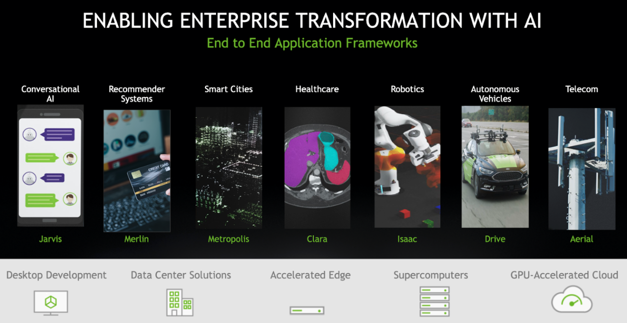
In May, NVIDIA announced two application frameworks, Jarvis for conversational AI and Merlin for recommendation systems. Merlin includes the HugeCTR framework for training that powered the latest MLPerf results.

These are part of a growing family of application frameworks for markets including automotive (NVIDIA DRIVE), healthcare (Clara), robotics (Isaac) and retail/smart cities (Metropolis).

SDKs x1280
NVIDIA application frameworks simplify enterprise AI from development to deployment.

DGX SuperPOD Architecture Delivers Speed at Scale

NVIDIA ran MLPerf tests for systems on Selene, an internal cluster based on the DGX SuperPOD, its public reference architecture for large-scale GPU clusters that can be deployed in weeks. That architecture extends the design principles and best practices used in the DGX POD to serve the most challenging problems in AI today.

Selene recently debuted on the TOP500 list as the fastest industrial system in the U.S. with more than an exaflops of AI performance. It’s also the world’s second most power-efficient system on the Green500 list.

Customers are already using these reference architectures to build DGX PODs and DGX SuperPODs of their own. They include HiPerGator, the fastest academic AI supercomputer in the U.S., which the University of Florida will feature as the cornerstone of its cross-curriculum AI initiative.

Meanwhile, a top supercomputing center, Argonne National Laboratory, is using DGX A100 to find ways to fight COVID-19. Argonne was the first of a half-dozen high performance computing centers to adopt A100 GPUs.

DGX POD Users x1280
Many users have adopted NVIDIA DGX PODs.

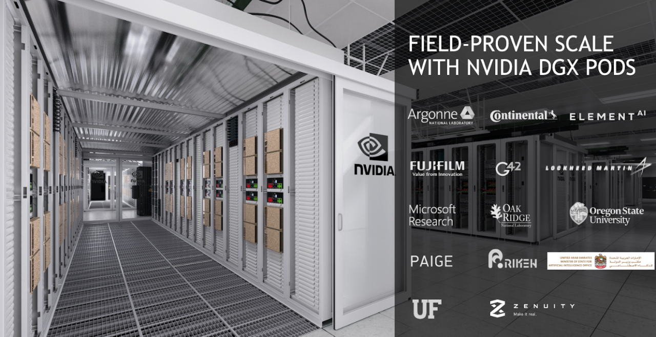
DGX SuperPODs are already driving business results for companies like Continental in automotive, Lockheed Martin in aerospace and Microsoft in cloud-computing services.

These systems are all up and running thanks in part to a broad ecosystem supporting NVIDIA GPUs and DGX systems.

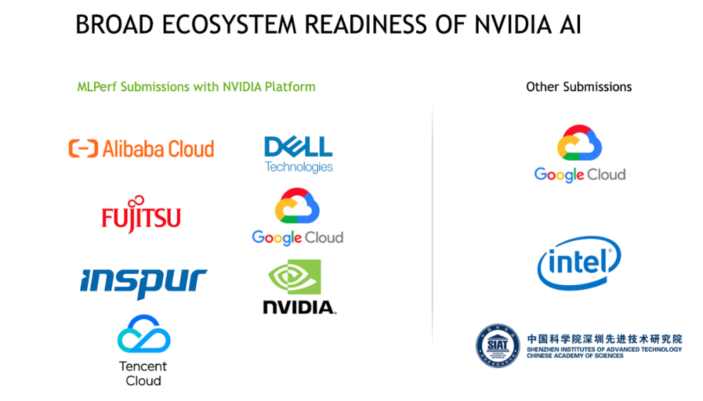
Strong MLPerf Showing by NVIDIA Ecosystem

Of the nine companies submitting results, seven submitted with NVIDIA GPUs including cloud service providers (Alibaba Cloud, Google Cloud, Tencent Cloud) and server makers (Dell, Fujitsu, and Inspur), highlighting the strength of NVIDIA’s ecosystem.

NVIDIA AI Ecosystem x1000
Many partners leveraged the NVIDIA AI platform for MLPerf submissions.

Many of these partners used containers on NGC, NVIDIA’s software hub, along with publicly available frameworks for their submissions.

The MLPerf partners represent part of an ecosystem of nearly two dozen cloud-service providers and OEMs with products or plans for online instances, servers and PCIe cards using NVIDIA A100 GPUs.

Test-Proven Software Available on NGC Today

Much of the same software NVIDIA and its partners used for the latest MLPerf benchmarks is available to customers today on NGC.

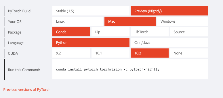
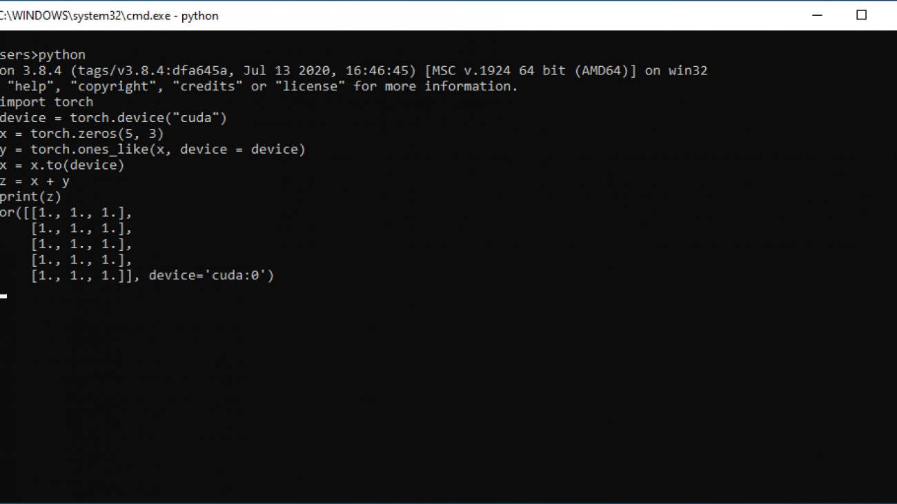
NGC is host to several GPU-optimized containers, software scripts, pre-trained models and SDKs. They empower data scientists and developers to accelerate their AI workflows across popular frameworks such as TensorFlow and PyTorch.

Organizations are embracing containers to save time getting to business results that matter. In the end, that’s the most important benchmark of all.

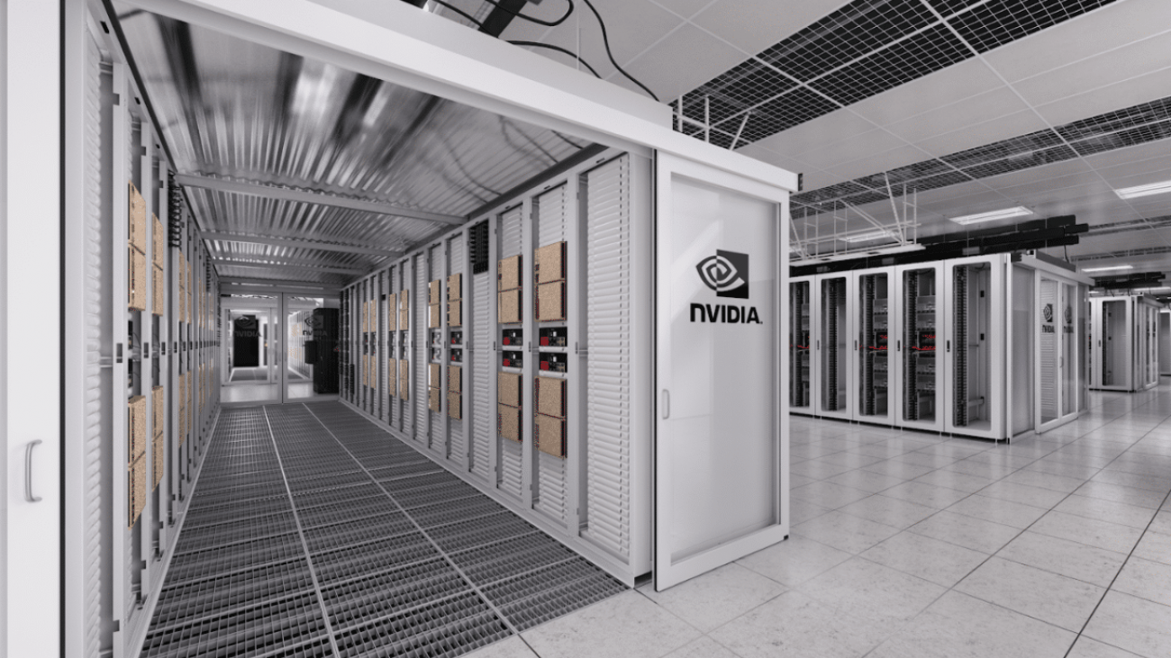
Artist’s rendering at top: NVIDIA’s new DGX SuperPOD, built in less than a month and featuring more than 2,000 NVIDIA A100 GPUs, swept every MLPerf benchmark category for at-scale performance among commercially available products. 

The post NVIDIA Breaks 16 AI Performance Records in Latest MLPerf Benchmarks appeared first on The Official NVIDIA Blog.

Read More

Algorithm finds hidden connections between paintings at the Met

Art is often heralded as the greatest journey into the past, solidifying a moment in time and space; the beautiful vehicle that lets us momentarily escape the present. 

With the boundless treasure trove of paintings that exist, the connections between these works of art from different periods of time and space can often go overlooked. It’s impossible for even the most knowledgeable of art critics to take in millions of paintings across thousands of years and be able to find unexpected parallels in themes, motifs, and visual styles. 

To streamline this process, a group of researchers from MIT’s Computer Science and Artificial Intelligence Laboratory (CSAIL) and Microsoft created an algorithm to discover hidden connections between paintings at the Metropolitan Museum of Art (the Met) and Amsterdam’s Rijksmuseum. 

Inspired by a special exhibit “Rembrandt and Velazquez” in the Rijksmuseum, the new “MosAIc” system finds paired or “analogous” works from different cultures, artists, and media by using deep networks to understand how “close” two images are. In that exhibit, the researchers were inspired by an unlikely, yet similar pairing: Francisco de Zurbarán’s “The Martyrdom of Saint Serapion” and Jan Asselijn’s “The Threatened Swan,” two works that portray scenes of profound altruism with an eerie visual resemblance.

“These two artists did not have a correspondence or meet each other during their lives, yet their paintings hinted at a rich, latent structure that underlies both of their works,” says CSAIL PhD student Mark Hamilton, the lead author on a paper about “MosAIc.” 

To find two similar paintings, the team used a new algorithm for image search to unearth the closest match by a particular artist or culture. For example, in response to a query about “which musical instrument is closest to this painting of a blue-and-white dress,” the algorithm retrieves an image of a blue-and-white porcelain violin. These works are not only similar in pattern and form, but also draw their roots from a broader cultural exchange of porcelain between the Dutch and Chinese. 

“Image retrieval systems let users find images that are semantically similar to a query image, serving as the backbone of reverse image search engines and many product recommendation engines,” says Hamilton. “Restricting an image retrieval system to particular subsets of images can yield new insights into relationships in the visual world. We aim to encourage a new level of engagement with creative artifacts.” 

How it works 

For many, art and science are irreconcilable: one grounded in logic, reasoning, and proven truths, and the other motivated by emotion, aesthetics, and beauty. But recently, AI and art took on a new flirtation that, over the past 10 years, developed into something more serious. 

A large branch of this work, for example, has previously focused on generating new art using AI. There was the GauGAN project developed by researchers at MIT, NVIDIA, and the University of California at Berkeley; Hamilton and others’ previous GenStudio project; and even an AI-generated artwork that sold at Sotheby’s for $51,000

MosAIc, however, doesn’t aim to create new art so much as help explore existing art. One similar tool, Google’s “X Degrees of Separation,” finds paths of art that connect two works of art, but MosAIc differs in that it only requires a single image. Instead of finding paths, it uncovers connections in whatever culture or media the user is interested in, such as finding the shared artistic form of “Anthropoides paradisea” and “Seth Slaying a Serpent, Temple of Amun at Hibis.” 

Hamilton notes that building out their algorithm was a tricky endeavor, because they wanted to find images that were similar not just in color or style, but in meaning and theme. In other words, they’d want dogs to be close to other dogs, people to be close to other people, and so forth. To achieve this, they probe a deep network’s inner “activations” for each image in the combined open access collections of the Met and the Rijksmuseum. Distance between the “activations” of this deep network, which are commonly called “features,” was how they judged image similarity.

To find analogous images between different cultures, the team used a new image-search data structure called a “conditional KNN tree” that groups similar images together in a tree-like structure. To find a close match, they start at the tree’s “trunk” and follow the most promising “branch” until they are sure they’ve found the closest image. The data structure improves on its predecessors by allowing the tree to quickly “prune” itself to a particular culture, artist, or collection, quickly yielding answers to new types of queries.

What Hamilton and his colleagues found surprising was that this approach could also be applied to helping find problems with existing deep networks, related to the surge of “deepfakes” that have recently cropped up. They applied this data structure to find areas where probabilistic models, such as the generative adversarial networks (GANs) that are often used to create deepfakes, break down. They coined these problematic areas “blind spots,” and note that they give us insight into how GANs can be biased. Such blind spots further show that GANs struggle to represent particular areas of a dataset, even if most of their fakes can fool a human. 

Testing MosAIc 

The team evaluated MosAIc’s speed, and how closely it aligned with our human intuition about visual analogies.

For the speed tests, they wanted to make sure that their data structure provided value over simply searching through the collection with quick, brute-force search. 

To understand how well the system aligned with human intuitions, they made and released two new datasets for evaluating conditional image retrieval systems. One dataset challenged algorithms to find images with the same content even after they had been “stylized” with a neural style transfer method. The second dataset challenged algorithms to recover English letters across different fonts. A bit less than two-thirds of the time, MosAIc was able to recover the correct image in a single guess from a “haystack” of 5,000 images.

“Going forward, we hope this work inspires others to think about how tools from information retrieval can help other fields like the arts, humanities, social science, and medicine,” says Hamilton. “These fields are rich with information that has never been processed with these techniques and can be a source for great inspiration for both computer scientists and domain experts. This work can be expanded in terms of new datasets, new types of queries, and new ways to understand the connections between works.” 

Hamilton wrote the paper on MosAIc alongside Professor Bill Freeman and MIT undergraduates Stefanie Fu and Mindren Lu. The MosAIc website was built by MIT, Fu, Lu, Zhenbang Chen, Felix Tran, Darius Bopp, Margaret Wang, Marina Rogers, and Johnny Bui, at the Microsoft Garage winter externship program.

Read More

Announcing ScaNN: Efficient Vector Similarity Search

Announcing ScaNN: Efficient Vector Similarity Search

Posted by Philip Sun, Software Engineer, Google Research

Suppose one wants to search through a large dataset of literary works using queries that require an exact match of title, author, or other easily machine-indexable criteria. Such a task would be well suited for a relational database using a language such as SQL. However, if one wants to support more abstract queries, such as “Civil War poem,” it is no longer possible to rely on naive similarity metrics such as the number of words in common between two phrases. For example, the query “science fiction” is more related to “future” than it is to “earth science” despite the former having zero, and the latter having one, word in common with the query.

Machine learning (ML) has greatly improved computers’ abilities to understand language semantics and therefore answer these abstract queries. Modern ML models can transform inputs such as text and images into embeddings, high dimensional vectors trained such that more similar inputs cluster closer together. For a given query, we can therefore compute its embedding, and find the literary works whose embeddings are closest to the query’s. In this manner, ML has transformed an abstract and previously difficult-to-specify task into a rigorous mathematical one. However, a computational challenge remains: for a given query embedding, how does one quickly find the nearest dataset embeddings? The set of embeddings is often too large for exhaustive search and its high dimensionality makes pruning difficult.

In our ICML 2020 paper, “Accelerating Large-Scale Inference with Anisotropic Vector Quantization,” we address this problem by focusing on how to compress the dataset vectors to enable fast approximate distance computations, and propose a new compression technique that significantly boosts accuracy compared to prior works. This technique is utilized in our recently open-sourced vector similarity search library (ScaNN), and enables us to outperform other vector similarity search libraries by a factor of two, as measured on ann-benchmarks.com.

The Importance of Vector Similarity Search
Embedding-based search is a technique that is effective at answering queries that rely on semantic understanding rather than simple indexable properties. In this technique, machine learning models are trained to map the queries and database items to a common vector embedding space, such that the distance between embeddings carries semantic meaning, i.e., similar items are closer together.

The two-tower neural network model, illustrated above, is a specific type of embedding-based search where queries and database items are mapped to the embedding space by two respective neural networks. In this example the model responds to natural-language queries for a hypothetical literary database.

To answer a query with this approach, the system must first map the query to the embedding space. It then must find, among all database embeddings, the ones closest to the query; this is the nearest neighbor search problem. One of the most common ways to define the query-database embedding similarity is by their inner product; this type of nearest neighbor search is known as maximum inner-product search (MIPS).

Because the database size can easily be in the millions or even billions, MIPS is often the computational bottleneck to inference speed, and exhaustive search is impractical. This necessitates the use of approximate MIPS algorithms that exchange some accuracy for a significant speedup over brute-force search.

A New Quantization Approach for MIPS
Several state-of-the-art solutions for MIPS are based on compressing the database items so that an approximation of their inner product can be computed in a fraction of the time taken by brute-force. This compression is commonly done with learned quantization, where a codebook of vectors is trained from the database and is used to approximately represent the database elements.

Previous vector quantization schemes quantized database elements with the aim of minimizing the average distance between each vector x and its quantized form . While this is a useful metric, optimizing for this is not equivalent to optimizing nearest-neighbor search accuracy. The key idea behind our paper is that encodings with higher average distance may actually result in superior MIPS accuracy.

The intuition for our result is illustrated below. Suppose we have two database embeddings x1 and x2, and must quantize each to one of two centers: c1 or c2. Our goal is to quantize each xi to i such that the inner product <q, i> is as similar to the original inner product <q, xi> as possible. This can be visualized as making the magnitude of the projection of i onto q as similar as possible to the projection of xi onto q. In the traditional approach to quantization (left), we would pick the closest center for each xi, which leads to an incorrect relative ranking of the two points: <q, 1> is greater than <q, 2>, even though <q, x1> is less than <q, x2>! If we instead assign x1 to c1 and x2 to c2, we get the correct ranking. This is illustrated in the figure below.

The goal is to quantize each xi to i = c1 or i = c2. Traditional quantization (left) results in the incorrect ordering of x1 and x2 for this query. Even though our approach (right) chooses centers farther away from the data points, this in fact leads to lower inner product error and higher accuracy.

It turns out that direction matters as well as magnitude–even though c1 is farther from x1 than c2, c1 is offset from x1 in a direction almost entirely orthogonal to x1, while c2’s offset is parallel (for x2, the same situation applies but flipped). Error in the parallel direction is much more harmful in the MIPS problem because it disproportionately impacts high inner products, which by definition are the ones that MIPS is trying to estimate accurately.

Based on this intuition, we more heavily penalize quantization error that is parallel to the original vector. We refer to our novel quantization technique as anisotropic vector quantization due to the directional dependence of its loss function. The ability of this technique to trade increased quantization error of lower inner products in exchange for superior accuracy for high inner products is the key innovation and the source of its performance gains.

In the above diagrams, ellipses denote contours of equal loss. In anisotropic vector quantization, error parallel to the original data point x is penalized more.

Anisotropic Vector Quantization in ScaNN
Anisotropic vector quantization allows ScaNN to better estimate inner products that are likely to be in the top-k MIPS results and therefore achieve higher accuracy. On the glove-100-angular benchmark from ann-benchmarks.com, ScaNN outperformed eleven other carefully tuned vector similarity search libraries, handling roughly twice as many queries per second for a given accuracy as the next-fastest library.*

Recall@k is a commonly used metric for nearest neighbor search accuracy, which measures the proportion of the true nearest k neighbors that are present in an algorithm’s returned k neighbors. ScaNN (upper purple line) consistently achieves superior performance across various points of the speed-accuracy trade-off.

ScaNN is open-source software and you can try it yourself at GitHub. The library can be directly installed via Pip and has interfaces for both TensorFlow and Numpy inputs. Please see the GitHub repository for further instructions on installing and configuring ScaNN.

Conclusion
By modifying the vector quantization objective to align with the goals of MIPS, we achieve state-of-the-art performance on nearest neighbor search benchmarks, a key indicator of embedding-based search performance. Although anisotropic vector quantization is an important technique, we believe it is just one example of the performance gains achievable by optimizing algorithms for the end goal of improving search accuracy rather than an intermediate goal such as compression distortion.

Acknowledgements
This post reflects the work of the entire ScaNN team: David Simcha, Erik Lindgren, Felix Chern, Nathan Cordeiro, Ruiqi Guo, Sanjiv Kumar, and Zonglin Li. We’d also like to thank Dan Holtmann-Rice, Dave Dopson, and Felix Yu.


* ScaNN performs similarly well on the other datasets of ann-benchmarks.com, but the website currently shows outdated, lower numbers. See this pull request for more representative performance figures on other datasets.

Read More

How SNCF Réseau and Olexya migrated a Caffe2 vision pipeline to Managed Spot Training in Amazon SageMaker

How SNCF Réseau and Olexya migrated a Caffe2 vision pipeline to Managed Spot Training in Amazon SageMaker

This blog post is co-written by guest authors from SNCF and Olexya.

Transportation and logistics are fertile ground for machine learning (ML). In this post, we show how the French state-owned railway company Société Nationale des Chemins de fer Français (SNCF) uses ML from AWS with the help of its technology partner Olexya to research, develop, and deploy innovative computer vision solutions.

SNCF was founded in 1938 and employs more than 270,000 people. SNCF Réseau is a subsidiary of SNCF that manages and operates the infrastructure for the rail network. SNCF Réseau and its technology partner Olexya deploy innovative solutions to assist the operations of the infrastructure and keep the bar high for infrastructure safety and quality. The field teams detect anomalies in the infrastructure by using computer vision.

SNCF Réseau researchers have been doing ML for a long time. An SNCF Réseau team developed a computer vision detection model on premises using the Caffe2 deep learning framework. The scientists then reached out to SNCF Réseau technology partner Olexya to assist with the provisioning of GPU to support iteration on the model. To keep operational overhead low and productivity high while retaining full flexibility on the scientific code, Olexya decided to use Amazon SageMaker to orchestrate the training and inference of the Caffe2 model. The process involved the following steps:

  1. Custom Docker creation.
  2. Training configuration ingestion via an Amazon Simple Storage Service (Amazon S3) data channel.
  3. Cost-efficient training via Amazon SageMaker Spot GPU training.
  4. Cost-efficient inference with the Amazon SageMaker training API.

Custom docker creation

The team created a Docker image wrapping the original Caffe2 code that respected the Amazon SageMaker Docker specification. Amazon SageMaker can accommodate multiple data sources, and has advanced integration with Amazon S3. Datasets stored in Amazon S3 can be automatically ingested in training containers running on Amazon SageMaker. To be able to process training data available in Amazon S3, Olexya had to direct the training code to read from the associated local path opt/ml/input/data/<channel name>. Similarly, the model artifact writing location had to be set to opt/ml/model. That way, Amazon SageMaker can automatically compress and ship the trained model artifact to Amazon S3 when training is complete.

Training configuration ingestion via an Amazon S3 data channel

The original Caffe2 training code was parametrized with an exhaustive and flexible YAML configuration file, so that researchers could change model settings without altering the scientific code. This external file was easy to keep external and ingest at training time in the container via the use of data channels. Data channels are Amazon S3 ARNs passed to the Amazon SageMaker SDK at training time and ingested in the Amazon SageMaker container when training starts. Olexya configured the data channels to read via a copy (copy mode), which is the default configuration. It is also possible to stream the data via Unix pipes (Pipe mode).

Cost-efficient training via Amazon SageMaker Spot GPU training

The team configured training infrastructure to be an ml.p3.2xlarge GPU-accelerated compute instance. The Amazon SageMaker ml.p3.2xlarge compute instance is specifically adapted to deep learning computer vision workloads: it’s equipped with an NVIDIA V100 GPU featuring 5,120 cores and 16 GB of High-Bandwidth Memory (HBM), which enables the fast training of large models.

Furthermore, Amazon SageMaker training API calls were set with Managed Spot Instance usage activated, which contributed to a reported savings of 71% compared to the on-demand Amazon SageMaker price. Amazon SageMaker Managed Spot Training is an Amazon SageMaker feature that enables the use of Amazon Elastic Compute Cloud (Amazon EC2) Spot Instance capacity for training. Amazon EC2 Spot Instances allow you to purchase unused Amazon EC2 computer capacity at a highly-reduced rate. In Amazon SageMaker, Spot Instance usage is fully managed by the service, and you can invoke it by setting two training SDK parameters:

  • train_use_spot_instances=True to request usage of Amazon SageMaker Spot Instances
  • train_max_wait set to the maximal acceptable waiting time in seconds

Cost-efficient inference with the Amazon SageMaker training API

In this research initiative, inference interruptions and delayed instantiation were acceptable to the end-user. Consequently, to further optimize costs, the team also used the Amazon SageMaker training API to run inference code, so that managed Amazon SageMaker Spot Instances could be used for inference too. Using the training API came with the additional benefit of a simpler learning curve because the same API is used for both steps of the model life cycle.

Time and cost savings

By applying those four steps, Olexya successfully ported an on-premises Caffe2 deep computer vision detection model to Amazon SageMaker for both training and inference. More impressively, the team completed that onboarding in about 3 weeks, and reported that the training time of the model was reduced from 3 days to 10 hours! The team further estimated that Amazon SageMaker allows a 71% total cost of ownership (TCO) reduction compared the locally available on-premises GPU fleet. A number of extra optimization techniques could reduce the costs even more, such as intelligent hyperparameter search with Amazon SageMaker automatic model tuning and mixed-precision training with the deep learning frameworks that support it.

In addition to SNCF Réseau, numerous AWS customers operating in transportation and logistics have improved their operations and delivered innovation by applying ML to their business. For example:

  • The Dubai-based logistics company Aramex uses ML for address parsing and transit time prediction. The company reports having 150 models in use, doing 450,000 predictions per day.
  • Transport for New South Wales uses the cloud to predict patronage numbers across the entire transport network, which enables the agency to better plan workforce and asset utilization and improve customer satisfaction.
  • Korean Air launched innovative projects with Amazon SageMaker to help predict and preempt maintenance for its aircraft fleet.

Conclusion

Amazon SageMaker supports the whole ML development cycle, from annotation to production deployment and monitoring. As illustrated by the work of Olexya and SNCF Réseau, Amazon SageMaker is framework-agnostic and accommodates a variety of deep learning workloads and frameworks. Although Docker images and SDK objects have been created to closely support Sklearn, TensorFlow, PyTorch, MXNet, XGBoost, and Chainer, you can bring custom Docker containers to onboard virtually any framework, such as PaddlePaddle, Catboost, R, or Caffe2. If you are an ML practitioner, don’t hesitate to test the service, and let us know what you build!


About the Authors

Olivier Cruchant is a Machine Learning Specialist Solution Architect at AWS, based in Lyon, France. Olivier helps French customers – from small startups to large enterprises – develop and deploy production-grade machine learning applications. In his spare time, he enjoys reading research papers and exploring the wilderness with friends and family.


Samuel Descroix is head manager of the Geographic and Analytic Data department at SNCF Réseau. He is in charge of all project teams and infrastructures. To be able to answer to all new use cases, he is constantly looking for most innovative and most relevant solutions to manage growing volumes and needs of complex analysis.


Alain Rivero is Project Manager in the Technology and Digital Transformation (TTD) department within the General Industrial and Engineering Department of SNCF Réseau. He manages projects implementing in-depth learning solutions to detect defects on rolling stock and tracks to increase traffic safety and guide decision-making within maintenance teams. His research focuses on image processing methods, supervised and unsupervised learning and their applications.


Pierre-Yves Bonnefoy is data architect at Olexya, currently working for SNCF Réseau IT department. One of his main assignments is to provide environments and sets of datas for Data Scientists and Data Analysts to work on complex analysis, and to help them with software solutions. Thanks to his large range of skills in development and system architecture, he accelerated the deployment of the project on Sagemaker instances, rationalization of costs and optimization of performance.


Emeric Chaize is certified Solution Architect in Olexya, currently working for SNCF Réseau IT department. He is in charge of Data Migration Project for IT Data Departement, with the responsabilty of covering all needs and usages of the company in data analysis. He defines and plans deployment of all the needed infrastructure for projects and Data Scientists.

Read More

PyTorch 1.6 released w/ Native AMP Support, Microsoft joins as maintainers for Windows

Today, we’re announcing the availability of PyTorch 1.6, along with updated domain libraries. We are also excited to announce the team at Microsoft is now maintaining Windows builds and binaries and will also be supporting the community on GitHub as well as the PyTorch Windows discussion forums.

The PyTorch 1.6 release includes a number of new APIs, tools for performance improvement and profiling, as well as major updates to both distributed data parallel (DDP) and remote procedure call (RPC) based distributed training.
A few of the highlights include:

  1. Automatic mixed precision (AMP) training is now natively supported and a stable feature (See here for more details) – thanks for NVIDIA’s contributions;
  2. Native TensorPipe support now added for tensor-aware, point-to-point communication primitives built specifically for machine learning;
  3. Added support for complex tensors to the frontend API surface;
  4. New profiling tools providing tensor-level memory consumption information;
  5. Numerous improvements and new features for both distributed data parallel (DDP) training and the remote procedural call (RPC) packages.

Additionally, from this release onward, features will be classified as Stable, Beta and Prototype. Prototype features are not included as part of the binary distribution and are instead available through either building from source, using nightlies or via compiler flag. You can learn more about what this change means in the post here. You can also find the full release notes here.

Performance & Profiling

[Stable] Automatic Mixed Precision (AMP) Training

AMP allows users to easily enable automatic mixed precision training enabling higher performance and memory savings of up to 50% on Tensor Core GPUs. Using the natively supported torch.cuda.amp API, AMP provides convenience methods for mixed precision, where some operations use the torch.float32 (float) datatype and other operations use torch.float16 (half). Some ops, like linear layers and convolutions, are much faster in float16. Other ops, like reductions, often require the dynamic range of float32. Mixed precision tries to match each op to its appropriate datatype.

  • Design doc (Link)
  • Documentation (Link)
  • Usage examples (Link)

[Beta] Fork/Join Parallelism

This release adds support for a language-level construct as well as runtime support for coarse-grained parallelism in TorchScript code. This support is useful for situations such as running models in an ensemble in parallel, or running bidirectional components of recurrent nets in parallel, and allows the ability to unlock the computational power of parallel architectures (e.g. many-core CPUs) for task level parallelism.

Parallel execution of TorchScript programs is enabled through two primitives: torch.jit.fork and torch.jit.wait. In the below example, we parallelize execution of foo:

import torch
from typing import List

def foo(x):
    return torch.neg(x)

@torch.jit.script
def example(x):
    futures = [torch.jit.fork(foo, x) for _ in range(100)]
    results = [torch.jit.wait(future) for future in futures]
    return torch.sum(torch.stack(results))

print(example(torch.ones([])))
  • Documentation (Link)

[Beta] Memory Profiler

The torch.autograd.profiler API now includes a memory profiler that lets you inspect the tensor memory cost of different operators inside your CPU and GPU models.

Here is an example usage of the API:

import torch
import torchvision.models as models
import torch.autograd.profiler as profiler

model = models.resnet18()
inputs = torch.randn(5, 3, 224, 224)
with profiler.profile(profile_memory=True, record_shapes=True) as prof:
    model(inputs)

# NOTE: some columns were removed for brevity
print(prof.key_averages().table(sort_by="self_cpu_memory_usage", row_limit=10))
# ---------------------------  ---------------  ---------------  ---------------
# Name                         CPU Mem          Self CPU Mem     Number of Calls
# ---------------------------  ---------------  ---------------  ---------------
# empty                        94.79 Mb         94.79 Mb         123
# resize_                      11.48 Mb         11.48 Mb         2
# addmm                        19.53 Kb         19.53 Kb         1
# empty_strided                4 b              4 b              1
# conv2d                       47.37 Mb         0 b              20
# ---------------------------  ---------------  ---------------  ---------------

Distributed Training & RPC

[Beta] TensorPipe backend for RPC

PyTorch 1.6 introduces a new backend for the RPC module which leverages the TensorPipe library, a tensor-aware point-to-point communication primitive targeted at machine learning, intended to complement the current primitives for distributed training in PyTorch (Gloo, MPI, …) which are collective and blocking. The pairwise and asynchronous nature of TensorPipe lends itself to new networking paradigms that go beyond data parallel: client-server approaches (e.g., parameter server for embeddings, actor-learner separation in Impala-style RL, …) and model and pipeline parallel training (think GPipe), gossip SGD, etc.

# One-line change needed to opt in
torch.distributed.rpc.init_rpc(
    ...
    backend=torch.distributed.rpc.BackendType.TENSORPIPE,
)

# No changes to the rest of the RPC API
torch.distributed.rpc.rpc_sync(...)
  • Design doc (Link)
  • Documentation (Link)

[Beta] DDP+RPC

PyTorch Distributed supports two powerful paradigms: DDP for full sync data parallel training of models and the RPC framework which allows for distributed model parallelism. Previously, these two features worked independently and users couldn’t mix and match these to try out hybrid parallelism paradigms.

Starting in PyTorch 1.6, we’ve enabled DDP and RPC to work together seamlessly so that users can combine these two techniques to achieve both data parallelism and model parallelism. An example is where users would like to place large embedding tables on parameter servers and use the RPC framework for embedding lookups, but store smaller dense parameters on trainers and use DDP to synchronize the dense parameters. Below is a simple code snippet.

// On each trainer

remote_emb = create_emb(on="ps", ...)
ddp_model = DDP(dense_model)

for data in batch:
   with torch.distributed.autograd.context():
      res = remote_emb(data)
      loss = ddp_model(res)
      torch.distributed.autograd.backward([loss])
  • DDP+RPC Tutorial (Link)
  • Documentation (Link)
  • Usage Examples (Link)

[Beta] RPC – Asynchronous User Functions

RPC Asynchronous User Functions supports the ability to yield and resume on the server side when executing a user-defined function. Prior to this feature, when a callee processes a request, one RPC thread waits until the user function returns. If the user function contains IO (e.g., nested RPC) or signaling (e.g., waiting for another request to unblock), the corresponding RPC thread would sit idle waiting for these events. As a result, some applications have to use a very large number of threads and send additional RPC requests, which can potentially lead to performance degradation. To make a user function yield on such events, applications need to: 1) Decorate the function with the @rpc.functions.async_execution decorator; and 2) Let the function return a torch.futures.Future and install the resume logic as callbacks on the Future object. See below for an example:

@rpc.functions.async_execution
def async_add_chained(to, x, y, z):
    return rpc.rpc_async(to, torch.add, args=(x, y)).then(
        lambda fut: fut.wait() + z
    )

ret = rpc.rpc_sync(
    "worker1", 
    async_add_chained, 
    args=("worker2", torch.ones(2), 1, 1)
)
        
print(ret)  # prints tensor([3., 3.])
  • Tutorial for performant batch RPC using Asynchronous User Functions (Link)
  • Documentation (Link)
  • Usage examples (Link)

Frontend API Updates

[Beta] Complex Numbers

The PyTorch 1.6 release brings beta level support for complex tensors including torch.complex64 and torch.complex128 dtypes. A complex number is a number that can be expressed in the form a + bj, where a and b are real numbers, and j is a solution of the equation x^2 = −1. Complex numbers frequently occur in mathematics and engineering, especially in signal processing and the area of complex neural networks is an active area of research. The beta release of complex tensors will support common PyTorch and complex tensor functionality, plus functions needed by Torchaudio, ESPnet and others. While this is an early version of this feature, and we expect it to improve over time, the overall goal is provide a NumPy compatible user experience that leverages PyTorch’s ability to run on accelerators and work with autograd to better support the scientific community.

Updated Domain Libraries

torchvision 0.7

torchvision 0.7 introduces two new pretrained semantic segmentation models, FCN ResNet50 and DeepLabV3 ResNet50, both trained on COCO and using smaller memory footprints than the ResNet101 backbone. We also introduced support for AMP (Automatic Mixed Precision) autocasting for torchvision models and operators, which automatically selects the floating point precision for different GPU operations to improve performance while maintaining accuracy.

  • Release notes (Link)

torchaudio 0.6

torchaudio now officially supports Windows. This release also introduces a new model module (with wav2letter included), new functionals (contrast, cvm, dcshift, overdrive, vad, phaser, flanger, biquad), datasets (GTZAN, CMU), and a new optional sox backend with support for TorchScript.

  • Release notes (Link)

Additional updates

HACKATHON

The Global PyTorch Summer Hackathon is back! This year, teams can compete in three categories virtually:

  1. PyTorch Developer Tools: Tools or libraries designed to improve productivity and efficiency of PyTorch for researchers and developers
  2. Web/Mobile Applications powered by PyTorch: Applications with web/mobile interfaces and/or embedded devices powered by PyTorch
  3. PyTorch Responsible AI Development Tools: Tools, libraries, or web/mobile apps for responsible AI development

This is a great opportunity to connect with the community and practice your machine learning skills.

LPCV Challenge

The 2020 CVPR Low-Power Vision Challenge (LPCV) – Online Track for UAV video submission deadline is coming up shortly. You have until July 31, 2020 to build a system that can discover and recognize characters in video captured by an unmanned aerial vehicle (UAV) accurately using PyTorch and Raspberry Pi 3B+.

Prototype Features

To reiterate, Prototype features in PyTorch are early features that we are looking to gather feedback on, gauge the usefulness of and improve ahead of graduating them to Beta or Stable. The following features are not part of the PyTorch 1.6 release and instead are available in nightlies with separate docs/tutorials to help facilitate early usage and feedback.

Distributed RPC/Profiler

Allow users to profile training jobs that use torch.distributed.rpc using the autograd profiler, and remotely invoke the profiler in order to collect profiling information across different nodes. The RFC can be found here and a short recipe on how to use this feature can be found here.

TorchScript Module Freezing

Module Freezing is the process of inlining module parameters and attributes values into the TorchScript internal representation. Parameter and attribute values are treated as final value and they cannot be modified in the frozen module. The PR for this feature can be found here and a short tutorial on how to use this feature can be found here.

Graph Mode Quantization

Eager mode quantization requires users to make changes to their model, including explicitly quantizing activations, module fusion, rewriting use of torch ops with Functional Modules and quantization of functionals are not supported. If we can trace or script the model, then the quantization can be done automatically with graph mode quantization without any of the complexities in eager mode, and it is configurable through a qconfig_dict. A tutorial on how to use this feature can be found here.

Quantization Numerical Suite

Quantization is good when it works, but it’s difficult to know what’s wrong when it doesn’t satisfy the expected accuracy. A prototype is now available for a Numerical Suite that measures comparison statistics between quantized modules and float modules. This is available to test using eager mode and on CPU only with more support coming. A tutorial on how to use this feature can be found here.

Cheers!

Team PyTorch

Read More

PyTorch feature classification changes

PyTorch feature classification changes

Traditionally features in PyTorch were classified as either stable or experimental with an implicit third option of testing bleeding edge features by building master or through installing nightly builds (available via prebuilt whls). This has, in a few cases, caused some confusion around the level of readiness, commitment to the feature and backward compatibility that can be expected from a user perspective. Moving forward, we’d like to better classify the 3 types of features as well as define explicitly here what each mean from a user perspective.

New Feature Designations

We will continue to have three designations for features but, as mentioned, with a few changes: Stable, Beta (previously Experimental) and Prototype (previously Nightlies). Below is a brief description of each and a comment on the backward compatibility expected:

Stable

Nothing changes here. A stable feature means that the user value-add is or has been proven, the API isn’t expected to change, the feature is performant and all documentation exists to support end user adoption.

Level of commitment: We expect to maintain these features long term and generally there should be no major performance limitations, gaps in documentation and we also expect to maintain backwards compatibility (although breaking changes can happen and notice will be given one release ahead of time).

Beta

We previously called these features ‘Experimental’ and we found that this created confusion amongst some of the users. In the case of a Beta level features, the value add, similar to a Stable feature, has been proven (e.g. pruning is a commonly used technique for reducing the number of parameters in NN models, independent of the implementation details of our particular choices) and the feature generally works and is documented. This feature is tagged as Beta because the API may change based on user feedback, because the performance needs to improve or because coverage across operators is not yet complete.

Level of commitment: We are committing to seeing the feature through to the Stable classification. We are however not committing to Backwards Compatibility. Users can depend on us providing a solution for problems in this area going forward, but the APIs and performance characteristics of this feature may change.

Prototype

Previously these were features that were known about by developers who paid close attention to RFCs and to features that land in master. In this case the feature is not available as part of binary distributions like PyPI or Conda (except maybe behind run-time flags), but we would like to get high bandwidth partner feedback ahead of a real release in order to gauge utility and any changes we need to make to the UX. To test these kinds of features we would, depending on the feature, recommend building from master or using the nightly whls that are made available on pytorch.org. For each prototype feature, a pointer to draft docs or other instructions will be provided.

Level of commitment: We are committing to gathering high bandwidth feedback only. Based on this feedback and potential further engagement between community members, we as a community will decide if we want to upgrade the level of commitment or to fail fast. Additionally, while some of these features might be more speculative (e.g. new Frontend APIs), others have obvious utility (e.g. model optimization) but may be in a state where gathering feedback outside of high bandwidth channels is not practical, e.g. the feature may be in an earlier state, may be moving fast (PRs are landing too quickly to catch a major release) and/or generally active development is underway.

What changes for current features?

First and foremost, you can find these designations on pytorch.org/docs. We will also be linking any early stage features here for clarity.

Additionally, the following features will be reclassified under this new rubric:

  1. High Level Autograd APIs: Beta (was Experimental)
  2. Eager Mode Quantization: Beta (was Experimental)
  3. Named Tensors: Prototype (was Experimental)
  4. TorchScript/RPC: Prototype (was Experimental)
  5. Channels Last Memory Layout: Beta (was Experimental)
  6. Custom C++ Classes: Beta (was Experimental)
  7. PyTorch Mobile: Beta (was Experimental)
  8. Java Bindings: Beta (was Experimental)
  9. Torch.Sparse: Beta (was Experimental)

Cheers,

Joe, Greg, Woo & Jessica

Read More

Microsoft becomes maintainer of the Windows version of PyTorch

Microsoft becomes maintainer of the Windows version of PyTorch

Along with the PyTorch 1.6 release, we are excited to announce that Microsoft has expanded its participation in the PyTorch community and is taking ownership of the development and maintenance of the PyTorch build for Windows.

According to the latest Stack Overflow developer survey, Windows remains the primary operating system for the developer community (46% Windows vs 28% MacOS). Jiachen Pu initially made a heroic effort to add support for PyTorch on Windows, but due to limited resources, Windows support for PyTorch has lagged behind other platforms. Lack of test coverage resulted in unexpected issues popping up every now and then. Some of the core tutorials, meant for new users to learn and adopt PyTorch, would fail to run. The installation experience was also not as smooth, with the lack of official PyPI support for PyTorch on Windows. Lastly, some of the PyTorch functionality was simply not available on the Windows platform, such as the TorchAudio domain library and distributed training support. To help alleviate this pain, Microsoft is happy to bring its Windows expertise to the table and bring PyTorch on Windows to its best possible self.

In the PyTorch 1.6 release, we have improved the core quality of the Windows build by bringing test coverage up to par with Linux for core PyTorch and its domain libraries and by automating tutorial testing. Thanks to the broader PyTorch community, which contributed TorchAudio support to Windows, we were able to add test coverage to all three domain libraries: TorchVision, TorchText and TorchAudio. In subsequent releases of PyTorch, we will continue improving the Windows experience based on community feedback and requests. So far, the feedback we received from the community points to distributed training support and a better installation experience using pip as the next areas of improvement.

In addition to the native Windows experience, Microsoft released a preview adding GPU compute support to Windows Subsystem for Linux (WSL) 2 distros, with a focus on enabling AI and ML developer workflows. WSL is designed for developers that want to run any Linux based tools directly on Windows. This preview enables valuable scenarios for a variety of frameworks and Python packages that utilize NVIDIA CUDA for acceleration and only support Linux. This means WSL customers using the preview can run native Linux based PyTorch applications on Windows unmodified without the need for a traditional virtual machine or a dual boot setup.

Getting started with PyTorch on Windows

It’s easy to get started with PyTorch on Windows. To install PyTorch using Anaconda with the latest GPU support, run the command below. To install different supported configurations of PyTorch, refer to the installation instructions on pytorch.org.

conda install pytorch torchvision cudatoolkit=10.2 -c pytorch

Once you install PyTorch, learn more by visiting the PyTorch Tutorials and documentation.

Getting started with PyTorch on Windows Subsystem for Linux

The preview of NVIDIA CUDA support in WSL is now available to Windows Insiders running Build 20150 or higher. In WSL, the command to install PyTorch using Anaconda is the same as the above command for native Windows. If you prefer pip, use the command below.

pip install torch torchvision

You can use the same tutorials and documentation inside your WSL environment as on native Windows. This functionality is still in preview so if you run into issues with WSL please share feedback via the WSL GitHub repo or with NVIDIA CUDA support share via NVIDIA’s Community Forum for CUDA on WSL.

Feedback

If you find gaps in the PyTorch experience on Windows, please let us know on the PyTorch discussion forum or file an issue on GitHub using the #module: windows label.

Read More

Introducing native PyTorch automatic mixed precision for faster training on NVIDIA GPUs

Introducing native PyTorch automatic mixed precision for faster training on NVIDIA GPUs

Most deep learning frameworks, including PyTorch, train with 32-bit floating point (FP32) arithmetic by default. However this is not essential to achieve full accuracy for many deep learning models. In 2017, NVIDIA researchers developed a methodology for mixed-precision training, which combined single-precision (FP32) with half-precision (e.g. FP16) format when training a network, and achieved the same accuracy as FP32 training using the same hyperparameters, with additional performance benefits on NVIDIA GPUs:

  • Shorter training time;
  • Lower memory requirements, enabling larger batch sizes, larger models, or larger inputs.

In order to streamline the user experience of training in mixed precision for researchers and practitioners, NVIDIA developed Apex in 2018, which is a lightweight PyTorch extension with Automatic Mixed Precision (AMP) feature. This feature enables automatic conversion of certain GPU operations from FP32 precision to mixed precision, thus improving performance while maintaining accuracy.

For the PyTorch 1.6 release, developers at NVIDIA and Facebook moved mixed precision functionality into PyTorch core as the AMP package, torch.cuda.amp. torch.cuda.amp is more flexible and intuitive compared to apex.amp. Some of apex.amp’s known pain points that torch.cuda.amp has been able to fix:

  • Guaranteed PyTorch version compatibility, because it’s part of PyTorch
  • No need to build extensions
  • Windows support
  • Bitwise accurate saving/restoring of checkpoints
  • DataParallel and intra-process model parallelism (although we still recommend torch.nn.DistributedDataParallel with one GPU per process as the most performant approach)
  • Gradient penalty (double backward)
  • torch.cuda.amp.autocast() has no effect outside regions where it’s enabled, so it should serve cases that formerly struggled with multiple calls to apex.amp.initialize() (including cross-validation) without difficulty. Multiple convergence runs in the same script should each use a fresh GradScaler instance, but GradScalers are lightweight and self-contained so that’s not a problem.
  • Sparse gradient support

With AMP being added to PyTorch core, we have started the process of deprecating apex.amp. We have moved apex.amp to maintenance mode and will support customers using apex.amp. However, we highly encourage apex.amp customers to transition to using torch.cuda.amp from PyTorch Core.

Example Walkthrough

Please see official docs for usage:

Example:

import torch 
# Creates once at the beginning of training 
scaler = torch.cuda.amp.GradScaler() 
 
for data, label in data_iter: 
   optimizer.zero_grad() 
   # Casts operations to mixed precision 
   with torch.cuda.amp.autocast(): 
      loss = model(data) 
 
   # Scales the loss, and calls backward() 
   # to create scaled gradients 
   scaler.scale(loss).backward() 
 
   # Unscales gradients and calls 
   # or skips optimizer.step() 
   scaler.step(optimizer) 
 
   # Updates the scale for next iteration 
   scaler.update() 

Performance Benchmarks

In this section, we discuss the accuracy and performance of mixed precision training with AMP on the latest NVIDIA GPU A100 and also previous generation V100 GPU. The mixed precision performance is compared to FP32 performance, when running Deep Learning workloads in the NVIDIA pytorch:20.06-py3 container from NGC.

Accuracy: AMP (FP16), FP32

The advantage of using AMP for Deep Learning training is that the models converge to the similar final accuracy while providing improved training performance. To illustrate this point, for Resnet 50 v1.5 training, we see the following accuracy results where higher is better. Please note that the below accuracy numbers are sample numbers that are subject to run to run variance of up to 0.4%. Accuracy numbers for other models including BERT, Transformer, ResNeXt-101, Mask-RCNN, DLRM can be found at NVIDIA Deep Learning Examples Github.

Training accuracy: NVIDIA DGX A100 (8x A100 40GB)

 epochs  Mixed Precision Top 1(%)  TF32 Top1(%)
 90  76.93  76.85

Training accuracy: NVIDIA DGX-1 (8x V100 16GB)

 epochs  Mixed Precision Top 1(%)  FP32 Top1(%)
50 76.25 76.26
90 77.09 77.01
250 78.42 78.30

Speedup Performance:

FP16 on NVIDIA V100 vs. FP32 on V100

AMP with FP16 is the most performant option for DL training on the V100. In Table 1, we can observe that for various models, AMP on V100 provides a speedup of 1.5x to 5.5x over FP32 on V100 while converging to the same final accuracy.

Figure 2. Performance of mixed precision training on NVIDIA 8xV100 vs. FP32 training on 8xV100 GPU. Bars represent the speedup factor of V100 AMP over V100 FP32. The higher the better.

FP16 on NVIDIA A100 vs. FP16 on V100

AMP with FP16 remains the most performant option for DL training on the A100. In Figure 3, we can observe that for various models, AMP on A100 provides a speedup of 1.3x to 2.5x over AMP on V100 while converging to the same final accuracy.

Figure 3. Performance of mixed precision training on NVIDIA 8xA100 vs. 8xV100 GPU. Bars represent the speedup factor of A100 over V100. The higher the better.

Call to action

AMP provides a healthy speedup for Deep Learning training workloads on Nvidia Tensor Core GPUs, especially on the latest Ampere generation A100 GPUs. You can start experimenting with AMP enabled models and model scripts for A100, V100, T4 and other GPUs available at NVIDIA deep learning examples. NVIDIA PyTorch with native AMP support is available from the PyTorch NGC container version 20.06. We highly encourage existing apex.amp customers to transition to using torch.cuda.amp from PyTorch Core available in the latest PyTorch 1.6 release.

Read More

Looking into the black box

Deep learning systems are revolutionizing technology around us, from voice recognition that pairs you with your phone to autonomous vehicles that are increasingly able to see and recognize obstacles ahead. But much of this success involves trial and error when it comes to the deep learning networks themselves. A group of MIT researchers recently reviewed their contributions to a better theoretical understanding of deep learning networks, providing direction for the field moving forward.

“Deep learning was in some ways an accidental discovery,” explains Tommy Poggio, investigator at the McGovern Institute for Brain Research, director of the Center for Brains, Minds, and Machines (CBMM), and the Eugene McDermott Professor in Brain and Cognitive Sciences. “We still do not understand why it works. A theoretical framework is taking form, and I believe that we are now close to a satisfactory theory. It is time to stand back and review recent insights.”

Climbing data mountains

Our current era is marked by a superabundance of data — data from inexpensive sensors of all types, text, the internet, and large amounts of genomic data being generated in the life sciences. Computers nowadays ingest these multidimensional datasets, creating a set of problems dubbed the “curse of dimensionality” by the late mathematician Richard Bellman.

One of these problems is that representing a smooth, high-dimensional function requires an astronomically large number of parameters. We know that deep neural networks are particularly good at learning how to represent, or approximate, such complex data, but why? Understanding why could potentially help advance deep learning applications.

“Deep learning is like electricity after Volta discovered the battery, but before Maxwell,” explains Poggio, who is the founding scientific advisor of The Core, MIT Quest for Intelligence, and an investigator in the Computer Science and Artificial Intelligence Laboratory (CSAIL) at MIT. “Useful applications were certainly possible after Volta, but it was Maxwell’s theory of electromagnetism, this deeper understanding that then opened the way to the radio, the TV, the radar, the transistor, the computers, and the internet.”

The theoretical treatment by Poggio, Andrzej Banburski, and Qianli Liao points to why deep learning might overcome data problems such as “the curse of dimensionality.” Their approach starts with the observation that many natural structures are hierarchical. To model the growth and development of a tree doesn’t require that we specify the location of every twig. Instead, a model can use local rules to drive branching hierarchically. The primate visual system appears to do something similar when processing complex data. When we look at natural images — including trees, cats, and faces — the brain successively integrates local image patches, then small collections of patches, and then collections of collections of patches. 

“The physical world is compositional — in other words, composed of many local physical interactions,” explains Qianli Liao, an author of the study, and a graduate student in the Department of Electrical Engineering and Computer Science and a member of the CBMM. “This goes beyond images. Language and our thoughts are compositional, and even our nervous system is compositional in terms of how neurons connect with each other. Our review explains theoretically why deep networks are so good at representing this complexity.”

The intuition is that a hierarchical neural network should be better at approximating a compositional function than a single “layer” of neurons, even if the total number of neurons is the same. The technical part of their work identifies what “better at approximating” means and proves that the intuition is correct.

Generalization puzzle

There is a second puzzle about what is sometimes called the unreasonable effectiveness of deep networks. Deep network models often have far more parameters than data to fit them, despite the mountains of data we produce these days. This situation ought to lead to what is called “overfitting,” where your current data fit the model well, but any new data fit the model terribly. This is dubbed poor generalization in conventional models. The conventional solution is to constrain some aspect of the fitting procedure. However, deep networks do not seem to require this constraint. Poggio and his colleagues prove that, in many cases, the process of training a deep network implicitly “regularizes” the solution, providing constraints.

The work has a number of implications going forward. Though deep learning is actively being applied in the world, this has so far occurred without a comprehensive underlying theory. A theory of deep learning that explains why and how deep networks work, and what their limitations are, will likely allow development of even much more powerful learning approaches.

“In the long term, the ability to develop and build better intelligent machines will be essential to any technology-based economy,” explains Poggio. “After all, even in its current — still highly imperfect — state, deep learning is impacting, or about to impact, just about every aspect of our society and life.”

Read More

Building a multilingual question and answer bot with Amazon Lex

Building a multilingual question and answer bot with Amazon Lex

You can use Amazon Lex to build a question and answer chatbot. However, if you live in a non-English-speaking country or your business has global reach, you will want a multilingual bot to cater to all your users. This post describes how to achieve that by using the multi-language functionality of your question and answer bot (QnABot).

The QnABot can detect the predominant language in an interaction by using Amazon Comprehend, a natural language processing (NLP) service that uses machine learning to find insights and relationships in text.

The bot then uses Amazon Translate, a neural machine translation service to translate the question to English. Then it can return a preconfigured answer in the end user’s language or translate it back from the default English text.

Although QnABot allows the end-user to interact with an Amazon Lex bot using text or voice, the multilingual feature primarily supports text interactions. Multilingual voice interactions are currently limited to use with Alexa skills.

The solution consists of three easy steps:

  1. Configure the multi-language functionality.
  2. Set up the alternate curated answers in a different language.
  3. Configure your Alexa skill with multiple languages.

For instructions on creating and customizing your bot, see Create a Question and Answer Bot with Amazon Lex and Amazon Alexa or the Q&A Self-Paced Guide. You can also see the following videos on YouTube:

Prerequisites

To implement this solution, you must have an AWS account. If you don’t have a professional account, the AWS Free Tier lets you gain experience with the AWS platform, products, and services.

You also need to deploy QnABot. If you have not already done so, launch the QnABot on an AWS CloudFormation stack in one of the available Regions.

When specifying your stack name, include QnA in the name, for example, MultiLangQnABot.

After you successfully deploy your CloudFormation stack, complete the following steps:

  1. Open the content designer page of your chatbot.

If this is the first time accessing the chatbot design console, you can find the correct URL on the AWS CloudFormation console on the Output tab of your bot stack. Look for the value for the ContentDesignerURL key. You should also receive an email with temporary credentials to access the QnABot designer.

  1. On the designer page, choose the menu icon.
  2. Under Tools, choose Import.
  3. Expand the Examples/Extensions
  4. Next to blog-samples, choose Load.

Configuring the multi-language functionality

You are now ready to configure the multi-language functionality. Complete the following steps:

  1. In the content designer page, under Tools, choose Settings.
  2. For the ENABLE_MULTI_LANGUAGE_SUPPORT parameter, change the value from false to true.
  3. Choose Save.
  4. To test the bot, open the client webpage.
  5. From the designer page, under Tools, choose QnABot Client.
  6. Enter the following questions (in English, Spanish, and French):
    • How do I modify Q and A Bot content ?
    • ¿Cómo modifico el contenido de Q y A Bot ?
    • Comment modifier le contenu Q et A Bot ?

The chatbot answers each time in the language you used, as shown in the following animation.

The QnABot is successfully using Amazon Translate to translate the answer automatically into the user’s native language.

Setting up alternate curated answers in a different language

You might need to provide a more natural experience and want to add a curated answer in the native language of your choice. To further customize the translation for each question, you can use the {{handlebar}} functionality. The QnABot provides the {{handlebar}} function ifLang, which takes the locale as a quoted parameter. You can use any of the languages that Amazon Translate supports. For more information, see What Is Amazon Translate?

For example, to customize the translation in Spanish, the ifLang function uses es as the locale parameter. See the following code:

{{#ifLang 'es'}}
          Su traducción al español
{{/ifLang}}

Additionally, if an unknown language is detected, you can support that with a default response by using the defaultLang function. See the following code:

{{#defaultLang}}
          Your default language answer
{{/defaultLang}}

As an example, modify the question you used earlier. Go back to the content designer and complete the following steps:

  1. Under Tools, choose Edit.
  2. Select 001 and choose the pencil icon on the right.
  3. Replace the text in the answer with the following code:
    {{#ifLang 'es'}}
    Use las herramientas de 'Question and Test' de 'Content Designer' para encontrar sus documentos existentes y editarlos directamente en la consola. También puede exportar documentos existentes como un archivo JSON, realizar cambios en el archivo y volver a importar.
    {{/ifLang}}
    {{#ifLang 'fr'}}
    Utilisez les outils 'Question and Test' de 'Content Designer' pour trouver vos documents existants et les modifier directement dans la console. Vous pouvez également exporter des documents existants sous forme de fichier JSON, apporter des modifications au fichier et réimporter.
    {{/ifLang}}
    {{#defaultLang}} 
    Use the Content Designer Question and Test tools to find your existing documents and edit them directly in the console. You can also export existing documents as a JSON file, make changes to the file, and re-import.
    {{/defaultLang}}
    

    Multi-language and handlebars, in general, also support markdown answers. For example, you could modify the preceding code to highlight the name of the interface that isn’t translated. See the following code:

    {{#ifLang 'es'}}
    Use las herramientas de ***'Question and Test'*** de ***'Content Designer'*** para encontrar sus documentos existentes y editarlos directamente en la consola. También puede exportar documentos existentes como un archivo JSON, realizar cambios en el archivo y volver a importar.
    {{/ifLang}}
    {{#ifLang 'fr'}}
    Utilisez les outils ***'Question and Test'*** de ***'Content Designer'*** pour trouver vos documents existants et les modifier directement dans la console. Vous pouvez également exporter des documents existants sous forme de fichier JSON, apporter des modifications au fichier et réimporter.
    {{/ifLang}}
    {{#defaultLang}} 
    Use the ***Content Designer Question and Test*** tools to find your existing documents and edit them directly in the console. You can also export existing documents as a JSON file, make changes to the file, and re-import.
    {{/defaultLang}}
    

  4. Choose Advanced and enter the new code in the Markdown Answer box.

  5. Choose Update.

If you try to ask your questions again, the answers are different because the chatbot is using your curated version.

You can also import the sample or extension named Language / Multiple Language Support.

This adds two questions to the system: Language.000 and Language.001. The first question allows the end-user to set their preferred language explicitly; the latter resets the preferred language and allow the QnABot to choose the locale based on the automatically detected predominant language.

Debugging the answers in a different language

You can use the ENABLE_DEBUG_RESPONSES setting to see how local language questions are translated to English by QnABot, and to tune the content as needed to ensure QnABot finds the best answer to a non-English question.

Complete the following steps to set up and test:

  1. In the content designer page, under Tools, choose Settings.
  2. For the ENABLE_DEBUG_RESPONSES parameter, change the value from false to true.
  3. Choose Save.
  4. To test the bot, open the client webpage.
  5. From the designer page, under Tools, choose QnABot Client.
  6. Try one of the question we used before, you can read the translation and use this information to tune your answer.

Configuring your Alexa skill with multiple languages

You first need to create your Alexa skill. For instructions, see Create a Question and Answer Bot with Amazon Lex and Amazon Alexa.

When your Alexa skill is working, add the additional languages by completing the following steps:

  1. On the Alexa developer console, open your skill.
  2. From the drop-down menu with your default language, choose Language settings.
  3. Add all the languages you want to support and choose Save.
  4. Under CUSTOM, choose JSON Editor.
  5. Copy the JSON from the editor, switch to the other language you want to support, and enter it in the editor pane (this overwrites the default).
  6. Choose Save Model.
  7. Choose Invocation and change the invocation name.
  8. Choose Save Model.
  9. Repeat these steps for any language you want to support.
  10. Build the model.

Testing your Alexa skill

You can now test your Alexa skill in other languages.

  1. On the Alexa developer console, select your skill.
  2. Choose Test.
  3. Change the language and type the invocation name of your skill for that language.
  4. After Alexa gives her initial greeting, ask the question you used before or any other question you added in the content designer.

Alexa answers you in the selected language.

Now your multilingual chatbot can be published on your website or as an Alexa skill. To integrate the QnABot in your website, you can use lex-web-ui. For instructions, see Deploy a Web UI for your Chatbot.

Conclusion

This post shows you how to configure and use the out-of-the-box feature of your QnABot to localize answers in any language Amazon Translate supports. It is an inexpensive way to deploy a multi-language chatbot, and you don’t need to adapt it to accommodate new Amazon Lex features.

As of this writing, this approach works for text-based interactions only; support for voice is limited to use with Alexa skills only.

For more information about experimenting with the capabilities of QnABot, see the Q&A Self-Paced Guide.


About the Authors

Fabrizio is a Specialist Solutions Architect for Database and Analytics in the AWS Canada Public Sector team. He has worked in the analytics field for the last 20 years, and has recently, and quite by surprise, become a Hockey Dad after moving to Canada.


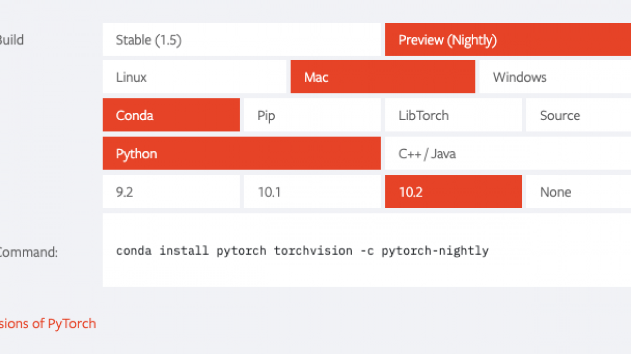
As a Solutions Architect at AWS supporting our Public Sector customers, Raj excites customers by showing them the art of the possible of what they can build on AWS and helps accelerate their innovation. Raj loves solving puzzles, mentoring, and supporting hackathons and seeing amazing ideas come to life.

Read More