Posts in category: Amazon AWS

AWS was delighted to present to and connect with over 18,000 in-person and 267,000 virtual attendees at NVIDIA GTC, a global artificial intelligence (AI) conference that took place March 2024 in San Jose, California, returning to a hybrid, in-person experience for the first time since 2019.

AWS has had a long-standing collaboration with NVIDIA for over 13 years. AWS was the first Cloud Service Provider (CSP) to offer NVIDIA GPUs in the public cloud, and remains among the first to deploy NVIDIA’s latest technologies.

Looking back at AWS re:Invent 2023, Jensen Huang, founder and CEO of NVIDIA, chatted with AWS CEO Adam Selipsky on stage, discussing how NVIDIA and AWS are working together to enable millions of developers to access powerful technologies needed to rapidly innovate with generative AI. NVIDIA is known for its cutting-edge accelerators and full-stack solutions that contribute to advancements in AI. The company is combining this expertise with the highly scalable, reliable, and secure AWS Cloud infrastructure to help customers run advanced graphics, machine learning, and generative AI workloads at an accelerated pace.

The collaboration between AWS and NVIDIA further expanded at GTC 2024, with the CEOs from both companies sharing their perspectives on the collaboration and state of AI in a press release:

“The deep collaboration between our two organizations goes back more than 13 years, when together we launched the world’s first GPU cloud instance on AWS, and today we offer the widest range of NVIDIA GPU solutions for customers,” says Adam Selipsky, CEO of AWS. “NVIDIA’s next-generation Grace Blackwell processor marks a significant step forward in generative AI and GPU computing. When combined with AWS’s powerful Elastic Fabric Adapter networking, Amazon EC2 UltraClusters’ hyper-scale clustering, and our unique AWS Nitro System’s advanced virtualization and security capabilities, we make it possible for customers to build and run multi-trillion parameter large language models faster, at massive scale, and more securely than anywhere else. Together, we continue to innovate to make AWS the best place to run NVIDIA GPUs in the cloud.”

“AI is driving breakthroughs at an unprecedented pace, leading to new applications, business models, and innovation across industries,” says Jensen Huang, founder and CEO of NVIDIA. “Our collaboration with AWS is accelerating new generative AI capabilities and providing customers with unprecedented computing power to push the boundaries of what’s possible.”

Joint announcements and keynote

On the first day of the NVIDIA GTC, AWS and NVIDIA made a joint announcement focused on their strategic collaboration to advance generative AI. Huang included the AWS and NVIDIA collaboration on a slide during his keynote, highlighting the following announcements. The GTC keynote had over 21 million views within the first 72 hours.

• AWS will offer the new NVIDIA Blackwell platform as Amazon Elastic Compute Cloud (Amazon EC2) instances and NVIDIA DGX Cloud to accelerate performance of building and running inference on multi-trillion parameter large language models (LLMs). Blackwell’s secure AI capabilities integrated with the AWS Nitro System and AWS Key Management Service (AWS KMS) will provide customers end-to-end control of their training data and model weights.
• AWS will provide the cloud infrastructure for Project Ceiba, an AI supercomputer built exclusively on AWS with NVIDIA DGX Cloud, which will feature 20,736 NVIDIA GB200 Grace Blackwell Superchips capable of 414 exaflops for NVIDIA’s own AI R&D.
• The Amazon SageMaker integration with NVIDIA NIM inference microservices will help customers further optimize price-performance of foundation models running on GPUs. (To learn more, see Optimize price-performance of LLM inference on NVIDIA GPUs using the Amazon SageMaker integration with NVIDIA NIM Microservices.)
• AWS HealthOmics with the NVIDIA BioNeMo platform will accelerate generative AI in biology and drug discovery. (To learn more, refer to NVIDIA BioNeMo Expands Computer-Aided Drug Discovery With New Foundation Models, Protein language model training with NVIDIA BioNeMo framework on AWS ParallelCluster, and Find the Next Blockbuster with NVIDIA BioNeMo Framework on Amazon SageMaker.)
• Amazon Robotics and NVIDIA’s long-standing collaboration regarding innovations in advanced simulations was also highlighted.

Media coverage

By March 22, AWS’s announcement with NVIDIA had generated 104 articles mentioning AWS and Amazon. The vast majority of coverage mentioned AWS’s plans to offer Blackwell-based instances. Adam Selipsky appeared on CNBC’s Mad Money to discuss the long-standing collaboration between AWS and NVIDIA, among the many other ways AWS is innovating in generative AI, stating that AWS has been the first to bring many of its GPUs to the cloud to drive efficiency and scalability for customers.

Project Ceiba has also been a focus in media coverage. Forbes referred to Project Ceiba as the “most exciting” project by AWS and NVIDIA, stating that it “should accelerate the pace of innovation in AI, making it possible to tackle more complex problems, develop more sophisticated models, and achieve previously unattainable breakthroughs.” The Next Platform ran an in-depth piece on Ceiba, stating that “the size and the aggregate compute of Ceiba cluster are both being radically expanded, which will give AWS a very large supercomputer in one of its data centers” and NVIDIA will use it to do AI research, among other things.

Live from GTC

“Live from GTC” was an on-site studio at GTC for invited speakers to have a fireside chat with tech influencers like VentureBeat. Chetan Kapoor, Director of Product Management for Amazon EC2 at AWS, was interviewed by VentureBeat at the Live from GTC studio, where he discussed AWS’s presence and highlighted key announcements at GTC.

The AWS booth and sessions

The AWS booth showcased generative AI services, like the LLMs with Anthropic and Cohere on Amazon Bedrock, PartyRock, Amazon Q, Amazon SageMaker JumpStart, and more. Highlights included:

• AWS AI Chess Robots – Two robotic arms playing chess against each other, with each move generated in the cloud with LLMs on Amazon Bedrock and powered by the NVIDIA Jetson platform and NVIDIA GPUs
• Wormhole – An alien robot from Media.Monks, who was busy having intelligent conversations with booth visitors powered by NVIDIA and a serverless Retrieval Augmented Generation (RAG) model using Claude 3 on Amazon Bedrock, along with other AWS services – Including SageMaker, Amazon Polly, and more
  
  Additionally, AWS had 10 GTC sessions showcasing how the latest technologies from AWS and NVIDIA can drive business outcomes using generative AI. Some highlights include:
• How Genius Sports Transforms NFL Game Viewing with Accelerated Computing on AWS (Presented by Amazon Web Services)
• Accelerate Time to Train Your Largest Generative AI Models With SageMaker HyperPod (Presented by Amazon Web Services)

AWS presence with partners and customers

During GTC, AWS invited 23 partner and customer solution demos to join its booth with either a dedicated demo kiosk or a 30-minute in-booth session. Such partners and customers included Ansys, Anthropic, Articul8, Bria.ai, Cohere, Deci, Deepbrain.AI, Denali Advanced Integration, Ganit, Hugging Face, Lilt, Linker Vision, Mavenir, MCE, Media.Monks, Modular, NVIDIA, Perplexity, Quantiphi, Run.ai, Salesforce, Second Spectrum, and Slalom.

Among them, high-potential early-stage startups in generative AI across the globe were showcased with a dedicated kiosk at the AWS booth. The AWS Startups team works closely with these companies by investing and supporting their growth, offering resources through programs like AWS Activate.

AWS Generative AI Competency

NVIDIA was one of the 45 launch partners for the new AWS Generative AI Competency program. The Generative AI Center of Excellence for AWS Partners team members were on site at the AWS booth, presenting this program for both existing and potential AWS partners. The program offers valuable resources along with best practices for all AWS partners to build, market, and sell generative AI solutions jointly with AWS.

Additional resources

Watch a video recap of the AWS presence at NVIDIA GTC 2024. For additional resources about the AWS and NVIDIA collaboration, refer to the AWS at NVIDIA GTC 2024 resource hub.

About the Author

Julie Tang is the Senior Global Partner Marketing Manager for Generative AI at Amazon Web Services (AWS), where she collaborates closely with NVIDIA to plan and execute partner marketing initiatives focused on generative AI. Throughout her tenure at AWS, she has held various partner marketing roles, including Global IoT Solutions, AWS Partner Solution Factory, and Sr. Campaign Manager in Americas Field Marketing. Prior to AWS, Julie served as the Marketing Director at Segway. She holds a Master’s degree in Communications Management with a focus on marketing and entertainment management from the University of Southern California, and dual Bachelor’s degrees in Law and Broadcast Journalism from Fudan University.

Read More

This blog post is co-written with Caroline Chung from Veoneer.

Veoneer is a global automotive electronics company and a world leader in automotive electronic safety systems. They offer best-in-class restraint control systems and have delivered over 1 billion electronic control units and crash sensors to car manufacturers globally. The company continues to build on a 70-year history of automotive safety development, specializing in cutting-edge hardware and systems that prevent traffic incidents and mitigate accidents.

Automotive in-cabin sensing (ICS) is an emerging space that uses a combination of several types of sensors such as cameras and radar, and artificial intelligence (AI) and machine learning (ML) based algorithms for enhancing safety and improving riding experience. Building such a system can be a complex task. Developers have to manually annotate large volumes of images for training and testing purposes. This is very time consuming and resource intensive. The turnaround time for such a task is several weeks. Furthermore, companies have to deal with issues such as inconsistent labels due to human errors.

AWS is focused on helping you increase your development speed and lower your costs for building such systems through advanced analytics like ML. Our vision is to use ML for automated annotation, enabling retraining of safety models, and ensuring consistent and reliable performance metrics. In this post, we share how, by collaborating with Amazon’s Worldwide Specialist Organization and the Generative AI Innovation Center, we developed an active learning pipeline for in-cabin image head bounding boxes and key points annotation. The solution reduces cost by over 90%, accelerates the annotation process from weeks to hours in terms of the turnaround time, and enables reusability for similar ML data labeling tasks.

Solution overview

Active learning is an ML approach that involves an iterative process of selecting and annotating the most informative data to train a model. Given a small set of labeled data and a large set of unlabeled data, active learning improves model performance, reduces labeling effort, and integrates human expertise for robust results. In this post, we build an active learning pipeline for image annotations with AWS services.

The following diagram demonstrates the overall framework for our active learning pipeline. The labeling pipeline takes images from an Amazon Simple Storage Service (Amazon S3) bucket and outputs annotated images with the cooperation of ML models and human expertise. The training pipeline preprocesses data and uses them to train ML models. The initial model is set up and trained on a small set of manually labeled data, and will be used in the labeling pipeline. The labeling pipeline and training pipeline can be iterated gradually with more labeled data to enhance the model’s performance.

In the labeling pipeline, an Amazon S3 Event Notification is invoked when a new batch of images comes into the Unlabeled Datastore S3 bucket, activating the labeling pipeline. The model produces the inference results on the new images. A customized judgement function selects parts of the data based on the inference confidence score or other user-defined functions. This data, with its inference results, is sent for a human labeling job on Amazon SageMaker Ground Truth created by the pipeline. The human labeling process helps annotate the data, and the modified results are combined with the remaining auto annotated data, which can be used later by the training pipeline.

Model retraining happens in the training pipeline, where we use the dataset containing the human-labeled data to retrain the model. A manifest file is produced to describe where the files are stored, and the same initial model is retrained on the new data. After retraining, the new model replaces the initial model, and the next iteration of the active learning pipeline starts.

Model deployment

Both the labeling pipeline and training pipeline are deployed on AWS CodePipeline. AWS CodeBuild instances are used for implementation, which is flexible and fast for a small amount of data. When speed is needed, we use Amazon SageMaker endpoints based on the GPU instance to allocate more resources to support and accelerate the process.

The model retraining pipeline can be invoked when there is new dataset or when the model’s performance needs improvement. One critical task in the retraining pipeline is to have the version control system for both the training data and the model. Although AWS services such as Amazon Rekognition have the integrated version control feature, which makes the pipeline straightforward to implement, customized models require metadata logging or additional version control tools.

The entire workflow is implemented using the AWS Cloud Development Kit (AWS CDK) to create necessary AWS components, including the following:

• Two roles for CodePipeline and SageMaker jobs
• Two CodePipeline jobs, which orchestrate the workflow
• Two S3 buckets for the code artifacts of the pipelines
• One S3 bucket for labeling the job manifest, datasets, and models
• Preprocessing and postprocessing AWS Lambda functions for the SageMaker Ground Truth labeling jobs

The AWS CDK stacks are highly modularized and reusable across different tasks. The training, inference code, and SageMaker Ground Truth template can be replaced for any similar active learning scenarios.

Model training

Model training includes two tasks: head bounding box annotation and human key points annotation. We introduce them both in this section.

Head bounding box annotation

Head bounding box annotation is a task to predict the location of a bounding box of the human head in an image. We use an Amazon Rekognition Custom Labels model for head bounding box annotations. The following sample notebook provides a step-by-step tutorial on how to train a Rekognition Custom Labels model via SageMaker.

We first need to prepare the data to start the training. We generate a manifest file for the training and a manifest file for the test dataset. A manifest file contains multiple items, each of which is for an image. The following is an example of the manifest file, which includes the image path, size, and annotation information:

{
    "source-ref": "s3://mlsl-sandox/rekognition_images/train/IMS_00000_00_000_000_R2_1900_01_01_00000_compressed_front_tof_amp_000.jpeg",
    "bounding-box-attribute-name": {
        "image_size": [{
                "width": 640,
                "height": 480,
                "depth": 3
            }
        ],
        "annotations": [{
                "class_id": 1,
                "top": 189,
                "left": 209,
                "width": 97,
                "height": 121
            }
        ]
    },
    "bounding-box-attribute-name-metadata": {
        "objects": [{
                "confidence": 1
            }
        ],
        "class-map": {
            "1": "Head"
        },
        "type": "groundtruth/object-detection",
        "human-annotated": "yes",
        "creation-date": "2023-04-07T20:04:42",
        "job-name": "testjob"
    }
}

Using the manifest files, we can load datasets to a Rekognition Custom Labels model for training and testing. We iterated the model with different amounts of training data and tested it on the same 239 unseen images. In this test, the mAP_50 score increased from 0.33 with 114 training images to 0.95 with 957 training images. The following screenshot shows the performance metrics of the final Rekognition Custom Labels model, which yields great performance in terms of F1 score, precision, and recall.

We further tested the model on a withheld dataset that has 1,128 images. The model consistently predicts accurate bounding box predictions on the unseen data, yielding a high mAP_50 of 94.9%. The following example shows an auto-annotated image with a head bounding box.

Key points annotation

Key points annotation produces locations of key points, including eyes, ears, nose, mouth, neck, shoulders, elbows, wrists, hips, and ankles. In addition to the location prediction, visibility of each point is needed to predict in this specific task, for which we design a novel method.

For key points annotation, we use a Yolo 8 Pose model on SageMaker as the initial model. We first prepare the data for training, including generating label files and a configuration .yaml file following Yolo’s requirements. After preparing the data, we train the model and save artifacts, including the model weights file. With the trained model weights file, we can annotate the new images.

In the training stage, all the labeled points with locations, including visible points and occluded points, are used for training. Therefore, this model by default provides the location and confidence of the prediction. In the following figure, a large confidence threshold (main threshold) near 0.6 is capable of dividing the points that are visible or occluded versus outside of camera’s viewpoints. However, occluded points and visible points are not separated by the confidence, which means the predicted confidence is not useful for predicting the visibility.

To get the prediction of visibility, we introduce an additional model trained on the dataset containing only visible points, excluding both occluded points and outside of camera’s viewpoints. The following figure shows the distribution of points with different visibility. Visible points and other points can be separated in the additional model. We can use a threshold (additional threshold) near 0.6 to get the visible points. By combining these two models, we design a method to predict the location and visibility.

A key point is first predicted by the main model with location and main confidence, then we get the additional confidence prediction from the additional model. Its visibility is then classified as follows:

• Visible, if its main confidence is greater than its main threshold, and its additional confidence is greater than the additional threshold
• Occluded, if its main confidence is greater than its main threshold, and its additional confidence is less than or equal to the additional threshold
• Outside of camera’s review, if otherwise

An example of key points annotation is demonstrated in the following image, where solid marks are visible points and hollow marks are occluded points. Outside of the camera’s review points are not shown.

Based on the standard OKS definition on the MS-COCO dataset, our method is able to achieve mAP_50​ of 98.4% on the unseen test dataset. In terms of visibility, the method yields a 79.2% classification accuracy on the same dataset.

Human labeling and retraining

Although the models achieve great performance on test data, there are still possibilities for making mistakes on new real-world data. Human labeling is the process to correct these mistakes for enhancing model performance using retraining. We designed a judgement function that combined the confidence value that output from the ML models for the output of all head bounding box or key points. We use the final score to identify these mistakes and the resultant bad labeled images, which need to be sent to the human labeling process.

In addition to bad labeled images, a small portion of images are randomly chosen for human labeling. These human-labeled images are added into the current version of the training set for retraining, enhancing model performance and overall annotation accuracy.

In the implementation, we use SageMaker Ground Truth for the human labeling process. SageMaker Ground Truth provides a user-friendly and intuitive UI for data labeling. The following screenshot demonstrates a SageMaker Ground Truth labeling job for head bounding box annotation.

The following screenshot demonstrates a SageMaker Ground Truth labeling job for key points annotation.

Cost, speed, and reusability

Cost and speed are the key advantages of using our solution compared to human labeling, as shown in the following tables. We use these tables to represent the cost savings and speed accelerations. Using the accelerated GPU SageMaker instance ml.g4dn.xlarge, the whole life training and inference cost on 100,000 images is 99% less than the cost of human labeling, while the speed is 10–10,000 times faster than the human labeling, depending on the task.

The first table summarizes the cost performance metrics.

The following table summarizes performance metrics.

Moreover, our solution provides reusability for similar tasks. Camera perception developments for other systems like advanced driver assist system (ADAS) and in-cabin systems can also adopt our solution.

Summary

In this post, we showed how to build an active learning pipeline for automatic annotation of in-cabin images utilizing AWS services. We demonstrate the power of ML, which enables you to automate and expedite the annotation process, and the flexibility of the framework that uses models either supported by AWS services or customized on SageMaker. With Amazon S3, SageMaker, Lambda, and SageMaker Ground Truth, you can streamline data storage, annotation, training, and deployment, and achieve reusability while reducing costs significantly. By implementing this solution, automotive companies can become more agile and cost-efficient by using ML-based advanced analytics such as automated image annotation.

Get started today and unlock the power of AWS services and machine learning for your automotive in-cabin sensing use cases!

About the Authors

Yanxiang Yu is an Applied Scientist at at the Amazon Generative AI Innovation Center. With over 9 years of experience building AI and machine learning solutions for industrial applications, he specializes in generative AI, computer vision, and time series modeling.

Tianyi Mao is an Applied Scientist at AWS based out of Chicago area. He has 5+ years of experience in building machine learning and deep learning solutions and focuses on computer vision and reinforcement learning with human feedbacks. He enjoys working with customers to understand their challenges and solve them by creating innovative solutions using AWS services.

Yanru Xiao is an Applied Scientist at the Amazon Generative AI Innovation Center, where he builds AI/ML solutions for customers’ real-world business problems. He has worked in several fields, including manufacturing, energy, and agriculture. Yanru obtained his Ph.D. in Computer Science from Old Dominion University.

Paul George is an accomplished product leader with over 15 years of experience in automotive technologies. He is adept at leading product management, strategy, Go-to-Market and systems engineering teams. He has incubated and launched several new sensing and perception products globally. At AWS, he is leading strategy and go-to-market for autonomous vehicle workloads.

Caroline Chung is an engineering manager at Veoneer (acquired by Magna International), she has over 14 years of experience developing sensing and perception systems. She currently leads interior sensing pre-development programs at Magna International managing a team of compute vision engineers and data scientists.

Read More

With Knowledge Bases for Amazon Bedrock, you can securely connect foundation models (FMs) in Amazon Bedrock to your company data for Retrieval Augmented Generation (RAG). Access to additional data helps the model generate more relevant, context-specific, and accurate responses without retraining the FMs.

In this post, we discuss two new features of Knowledge Bases for Amazon Bedrock specific to the RetrieveAndGenerate API: configuring the maximum number of results and creating custom prompts with a knowledge base prompt template. You can now choose these as query options alongside the search type.

Overview and benefits of new features

The maximum number of results option gives you control over the number of search results to be retrieved from the vector store and passed to the FM for generating the answer. This allows you to customize the amount of background information provided for generation, thereby giving more context for complex questions or less for simpler questions. It allows you to fetch up to 100 results. This option helps improve the likelihood of relevant context, thereby improving the accuracy and reducing the hallucination of the generated response.

The custom knowledge base prompt template allows you to replace the default prompt template with your own to customize the prompt that’s sent to the model for response generation. This allows you to customize the tone, output format, and behavior of the FM when it responds to a user’s question. With this option, you can fine-tune terminology to better match your industry or domain (such as healthcare or legal). Additionally, you can add custom instructions and examples tailored to your specific workflows.

In the following sections, we explain how you can use these features with either the AWS Management Console or SDK.

Prerequisites

To follow along with these examples, you need to have an existing knowledge base. For instructions to create one, see Create a knowledge base.

Configure the maximum number of results using the console

To use the maximum number of results option using the console, complete the following steps:

1. On the Amazon Bedrock console, choose Knowledge bases in the left navigation pane.
2. Select the knowledge base you created.
3. Choose Test knowledge base.
4. Choose the configuration icon.
5. Choose Sync data source before you start testing your knowledge base.
   
6. Under Configurations, for Search Type, select a search type based on your use case.

For this post, we use hybrid search because it combines semantic and text search to provider greater accuracy. To learn more about hybrid search, see Knowledge Bases for Amazon Bedrock now supports hybrid search.

7. Expand Maximum number of source chunks and set your maximum number of results.
   

To demonstrate the value of the new feature, we show examples of how you can increase the accuracy of the generated response. We used Amazon 10K document for 2023 as the source data for creating the knowledge base. We use the following query for experimentation: “In what year did Amazon’s annual revenue increase from $245B to $434B?”

The correct response for this query is “Amazon’s annual revenue increased from $245B in 2019 to $434B in 2022,” based on the documents in the knowledge base. We used Claude v2 as the FM to generate the final response based on the contextual information retrieved from the knowledge base. Claude 3 Sonnet and Claude 3 Haiku are also supported as the generation FMs.

We ran another query to demonstrate the comparison of retrieval with different configurations. We used the same input query (“In what year did Amazon’s annual revenue increase from $245B to $434B?”) and set the maximum number of results to 5.

As shown in the following screenshot, the generated response was “Sorry, I am unable to assist you with this request.”

Next, we set the maximum results to 12 and ask the same question. The generated response is “Amazon’s annual revenue increase from $245B in 2019 to $434B in 2022.”

As shown in this example, we are able to retrieve the correct answer based on the number of retrieved results. If you want to learn more about the source attribution that constitutes the final output, choose Show source details to validate the generated answer based on the knowledge base.

Customize a knowledge base prompt template using the console

You can also customize the default prompt with your own prompt based on the use case. To do so on the console, complete the following steps:

1. Repeat the steps in the previous section to start testing your knowledge base.
2. Enable Generate responses.
   
3. Select the model of your choice for response generation.

We use the Claude v2 model as an example in this post. The Claude 3 Sonnet and Haiku model is also available for generation.

4. Choose Apply to proceed.
   

After you choose the model, a new section called Knowledge base prompt template appears under Configurations.

5. Choose Edit to start customizing the prompt.
   
6. Adjust the prompt template to customize how you want to use the retrieved results and generate content.

For this post, we gave a few examples for creating a “Financial Advisor AI system” using Amazon financial reports with custom prompts. For best practices on prompt engineering, refer to Prompt engineering guidelines.

We now customize the default prompt template in several different ways, and observe the responses.

Let’s first try a query with the default prompt. We ask “What was the Amazon’s revenue in 2019 and 2021?” The following shows our results.

From the output, we find that it’s generating the free-form response based on the retrieved knowledge. The citations are also listed for reference.

Let’s say we want to give extra instructions on how to format the generated response, like standardizing it as JSON. We can add these instructions as a separate step after retrieving the information, as part of the prompt template:

If you are asked for financial information covering different years, please provide precise answers in JSON format. Use the year as the key and the concise answer as the value. For example: {year:answer}

The final response has the required structure.

By customizing the prompt, you can also change the language of the generated response. In the following example, we instruct the model to provide an answer in Spanish.

After removing $output_format_instructions$ from the default prompt, the citation from the generated response is removed.

In the following sections, we explain how you can use these features with the SDK.

Configure the maximum number of results using the SDK

To change the maximum number of results with the SDK, use the following syntax. For this example, the query is “In what year did Amazon’s annual revenue increase from $245B to $434B?” The correct response is “Amazon’s annual revenue increase from $245B in 2019 to $434B in 2022.”

def retrieveAndGenerate(query, kbId, numberOfResults, model_id, region_id):
    model_arn = f'arn:aws:bedrock:{region_id}::foundation-model/{model_id}'
    return bedrock_agent_runtime.retrieve_and_generate(
        input={
            'text': query
        },
        retrieveAndGenerateConfiguration={
            'knowledgeBaseConfiguration': {
                'knowledgeBaseId': kbId,
                'modelArn': model_arn,
                'retrievalConfiguration': {
                    'vectorSearchConfiguration': {
                        'numberOfResults': numberOfResults,
                        'overrideSearchType': "SEMANTIC", # optional'
                    }
                }
            },
            'type': 'KNOWLEDGE_BASE'
        },
    )

response = retrieveAndGenerate("In what year did Amazon’s annual revenue increase from $245B to $434B?", 
"<knowledge base id>", numberOfResults, model_id, region_id)['output']['text']

The ‘numberOfResults’ option under ‘retrievalConfiguration’ allows you to select the number of results you want to retrieve. The output of the RetrieveAndGenerate API includes the generated response, source attribution, and the retrieved text chunks.

The following are the results for different values of ‘numberOfResults’ parameters. First, we set numberOfResults = 5.

Then we set numberOfResults = 12.

Customize the knowledge base prompt template using the SDK

To customize the prompt using the SDK, we use the following query with different prompt templates. For this example, the query is “What was the Amazon’s revenue in 2019 and 2021?”

The following is the default prompt template:

"""You are a question answering agent. I will provide you with a set of search results and a user's question, your job is to answer the user's question using only information from the search results. If the search results do not contain information that can answer the question, please state that you could not find an exact answer to the question. Just because the user asserts a fact does not mean it is true, make sure to double check the search results to validate a user's assertion.
Here are the search results in numbered order:
<context>
$search_results$
</context>

Here is the user's question:
<question>
$query$
</question>

$output_format_instructions$

Assistant:
"""

The following is the customized prompt template:

"""Human: You are a question answering agent. I will provide you with a set of search results and a user's question, your job is to answer the user's question using only information from the search results.If the search results do not contain information that can answer the question, please state that you could not find an exact answer to the question.Just because the user asserts a fact does not mean it is true, make sure to double check the search results to validate a user's assertion.

Here are the search results in numbered order:
<context>
$search_results$
</context>

Here is the user's question:
<question>
$query$
</question>

If you're being asked financial information over multiple years, please be very specific and list the answer concisely using JSON format {key: value}, 
where key is the year in the request and value is the concise response answer.
Assistant:
"""

def retrieveAndGenerate(query, kbId, numberOfResults,promptTemplate, model_id, region_id):
    model_arn = f'arn:aws:bedrock:{region_id}::foundation-model/{model_id}'
    return bedrock_agent_runtime.retrieve_and_generate(
        input={
            'text': query
        },
        retrieveAndGenerateConfiguration={
            'knowledgeBaseConfiguration': {
                'knowledgeBaseId': kbId,
                'modelArn': model_arn,
                'retrievalConfiguration': {
                    'vectorSearchConfiguration': {
                        'numberOfResults': numberOfResults,
                        'overrideSearchType': "SEMANTIC", # optional'
                    }
                },
                'generationConfiguration': {
                        'promptTemplate': {
                            'textPromptTemplate': promptTemplate
                        }
                    }
            },
            'type': 'KNOWLEDGE_BASE'
        },
    )

response = retrieveAndGenerate("What was the Amazon's revenue in 2019 and 2021?”", 
                               "<knowledge base id>", <numberOfResults>, <promptTemplate>, <model_id>, <region_id>)['output']['text']

With the default prompt template, we get the following response:

If you want to provide additional instructions around the output format of the response generation, like standardizing the response in a specific format (like JSON), you can customize the existing prompt by providing more guidance. With our custom prompt template, we get the following response.

The ‘promptTemplate‘ option in ‘generationConfiguration‘ allows you to customize the prompt for better control over answer generation.

Conclusion

In this post, we introduced two new features in Knowledge Bases for Amazon Bedrock: adjusting the maximum number of search results and customizing the default prompt template for the RetrieveAndGenerate API. We demonstrated how to configure these features on the console and via SDK to improve performance and accuracy of the generated response. Increasing the maximum results provides more comprehensive information, whereas customizing the prompt template allows you to fine-tune instructions for the foundation model to better align with specific use cases. These enhancements offer greater flexibility and control, enabling you to deliver tailored experiences for RAG-based applications.

For additional resources to start implementing in your AWS environment, refer to the following:

• User guide: Knowledge bases for Amazon Bedrock
• YouTube video: Use RAG to improve responses in generative AI application
• GitHub repo code samples: Amazon Bedrock Knowledge Base – Samples for building RAG workflows

About the authors

Sandeep Singh is a Senior Generative AI Data Scientist at Amazon Web Services, helping businesses innovate with generative AI. He specializes in Generative AI, Artificial Intelligence, Machine Learning, and System Design. He is passionate about developing state-of-the-art AI/ML-powered solutions to solve complex business problems for diverse industries, optimizing efficiency and scalability.

Suyin Wang is an AI/ML Specialist Solutions Architect at AWS. She has an interdisciplinary education background in Machine Learning, Financial Information Service and Economics, along with years of experience in building Data Science and Machine Learning applications that solved real-world business problems. She enjoys helping customers identify the right business questions and building the right AI/ML solutions. In her spare time, she loves singing and cooking.

Sherry Ding is a senior artificial intelligence (AI) and machine learning (ML) specialist solutions architect at Amazon Web Services (AWS). She has extensive experience in machine learning with a PhD degree in computer science. She mainly works with public sector customers on various AI/ML related business challenges, helping them accelerate their machine learning journey on the AWS Cloud. When not helping customers, she enjoys outdoor activities.

Read More

At AWS re:Invent 2023, we announced the general availability of Knowledge Bases for Amazon Bedrock. With Knowledge Bases for Amazon Bedrock, you can securely connect foundation models (FMs) in Amazon Bedrock to your company data using a fully managed Retrieval Augmented Generation (RAG) model.

For RAG-based applications, the accuracy of the generated responses from FMs depend on the context provided to the model. Contexts are retrieved from vector stores based on user queries. In the recently released feature for Knowledge Bases for Amazon Bedrock, hybrid search, you can combine semantic search with keyword search. However, in many situations, you may need to retrieve documents created in a defined period or tagged with certain categories. To refine the search results, you can filter based on document metadata to improve retrieval accuracy, which in turn leads to more relevant FM generations aligned with your interests.

In this post, we discuss the new custom metadata filtering feature in Knowledge Bases for Amazon Bedrock, which you can use to improve search results by pre-filtering your retrievals from vector stores.

Metadata filtering overview

Prior to the release of metadata filtering, all semantically relevant chunks up to the pre-set maximum would be returned as context for the FM to use to generate a response. Now, with metadata filters, you can retrieve not only semantically relevant chunks but a well-defined subset of those relevant chucks based on applied metadata filters and associated values.

With this feature, you can now supply a custom metadata file (each up to 10 KB) for each document in the knowledge base. You can apply filters to your retrievals, instructing the vector store to pre-filter based on document metadata and then search for relevant documents. This way, you have control over the retrieved documents, especially if your queries are ambiguous. For example, you can use legal documents with similar terms for different contexts, or movies that have a similar plot released in different years. In addition, by reducing the number of chunks that are being searched over, you achieve performance advantages like a reduction in CPU cycles and cost of querying the vector store, in addition to improvement in accuracy.

To use the metadata filtering feature, you need to provide metadata files alongside the source data files with the same name as the source data file and .metadata.json suffix. Metadata can be string, number, or Boolean. The following is an example of the metadata file content:

{
    "metadataAttributes" : { 
        "tag" : "project EVE",
        "year" :  2016,
        "team": "ninjas"
    }
}

The metadata filtering feature of Knowledge Bases for Amazon Bedrock is available in AWS Regions US East (N. Virginia) and US West (Oregon).

The following are common use cases for metadata filtering:

• Document chatbot for a software company – This allows users to find product information and troubleshooting guides. Filters on the operating system or application version, for example, can help avoid retrieving obsolete or irrelevant documents.
• Conversational search of an organization’s application – This allows users to search through documents, kanbans, meeting recording transcripts, and other assets. Using metadata filters on work groups, business units, or project IDs, you can personalize the chat experience and improve collaboration. An example would be, “What is the status of project Sphinx and risks raised,” where users can filter documents for a specific project or source type (such as email or meeting documents).
• Intelligent search for software developers – This allows developers to look for information of a specific release. Filters on the release version, document type (such as code, API reference, or issue) can help pinpoint relevant documents.

Solution overview

In the following sections, we demonstrate how to prepare a dataset to use as a knowledge base, and then query with metadata filtering. You can query using either the AWS Management Console or SDK.

Prepare a dataset for Knowledge Bases for Amazon Bedrock

For this post, we use a sample dataset about fictional video games to illustrate how to ingest and retrieve metadata using Knowledge Bases for Amazon Bedrock. If you want to follow along in your own AWS account, download the file.

If you want to add metadata to your documents in an existing knowledge base, create the metadata files with the expected filename and schema, then skip to the step to sync your data with the knowledge base to start the incremental ingestion.

In our sample dataset, each game’s document is a separate CSV file (for example, s3://$bucket_name/video_game/$game_id.csv) with the following columns:

title, description, genres, year, publisher, score

Each game’s metadata has the suffix .metadata.json (for example, s3://$bucket_name/video_game/$game_id.csv.metadata.json) with the following schema:

{
  "metadataAttributes": {
    "id": number, 
    "genres": string,
    "year": number,
    "publisher": string,
    "score": number
  }
}

Create a knowledge base for Amazon Bedrock

For instructions to create a new knowledge base, see Create a knowledge base. For this example, we use the following settings:

• On the Set up data source page, under Chunking strategy, select No chunking, because you’ve already preprocessed the documents in the previous step.
• In the Embeddings model section, choose Titan G1 Embeddings – Text.
• In the Vector database section, choose Quick create a new vector store. The metadata filtering feature is available for all supported vector stores.

Synchronize the dataset with the knowledge base

After you create the knowledge base, and your data files and metadata files are in an Amazon Simple Storage Service (Amazon S3) bucket, you can start the incremental ingestion. For instructions, see Sync to ingest your data sources into the knowledge base.

Query with metadata filtering on the Amazon Bedrock console

To use the metadata filtering options on the Amazon Bedrock console, complete the following steps:

1. On the Amazon Bedrock console, choose Knowledge bases in the navigation pane.
2. Choose the knowledge base you created.
3. Choose Test knowledge base.
4. Choose the Configurations icon, then expand Filters.
5. Enter a condition using the format: key = value (for example, genres = Strategy) and press Enter.
6. To change the key, value, or operator, choose the condition.
   
7. Continue with the remaining conditions (for example, (genres = Strategy AND year >= 2023) OR (rating >= 9))
   
8. When finished, enter your query in the message box, then choose Run.

For this post, we enter the query “A strategy game with cool graphic released after 2023.”

Query with metadata filtering using the SDK

To use the SDK, first create the client for the Agents for Amazon Bedrock runtime:

import boto3

bedrock_agent_runtime = boto3.client(
    service_name = "bedrock-agent-runtime"
)

Then construct the filter (the following are some examples):

# genres = Strategy
single_filter= {
    "equals": {
        "key": "genres",
        "value": "Strategy"
    }
}

# genres = Strategy AND year >= 2023
one_group_filter= {
    "andAll": [
        {
            "equals": {
                "key": "genres",
                "value": "Strategy"
            }
        },
        {
            "GreaterThanOrEquals": {
                "key": "year",
                "value": 2023
            }
        }
    ]
}

# (genres = Strategy AND year >=2023) OR score >= 9
two_group_filter = {
    "orAll": [
        {
            "andAll": [
                {
                    "equals": {
                        "key": "genres",
                        "value": "Strategy"
                    }
                },
                {
                    "GreaterThanOrEquals": {
                        "key": "year",
                        "value": 2023
                    }
                }
            ]
        },
        {
            "GreaterThanOrEquals": {
                "key": "score",
                "value": "9"
            }
        }
    ]
}

Pass the filter to retrievalConfiguration of the Retrieval API or RetrieveAndGenerate API:

retrievalConfiguration={
        "vectorSearchConfiguration": {
            "filter": metadata_filter
        }
    }

The following table lists a few responses with different metadata filtering conditions.

In addition to custom metadata, you can also filter using S3 prefixes (which is a built-in metadata, so you don’t need to provide any metadata files). For example, if you organize the game documents into prefixes by publisher (for example, s3://$bucket_name/video_game/$publisher/$game_id.csv), you can filter with the specific publisher (for example, neo_tokyo_games) using the following syntax:

publisher_filter = {
    "startsWith": {
                    "key": "x-amz-bedrock-kb-source-uri",
                    "value": "s3://$bucket_name/video_game/neo_tokyo_games/"
                }
}

Clean up

To clean up your resources, complete the following steps:

1. Delete the knowledge base:
   1. On the Amazon Bedrock console, choose Knowledge bases under Orchestration in the navigation pane.
   2. Choose the knowledge base you created.
   3. Take note of the AWS Identity and Access Management (IAM) service role name in the Knowledge base overview section.
   4. In the Vector database section, take note of the collection ARN.
   5. Choose Delete, then enter delete to confirm.
2. Delete the vector database:
   1. On the Amazon OpenSearch Service console, choose Collections under Serverless in the navigation pane.
   2. Enter the collection ARN you saved in the search bar.
   3. Select the collection and chose Delete.
   4. Enter confirm in the confirmation prompt, then choose Delete.
3. Delete the IAM service role:
   1. On the IAM console, choose Roles in the navigation pane.
   2. Search for the role name you noted earlier.
   3. Select the role and choose Delete.
   4. Enter the role name in the confirmation prompt and delete the role.
4. Delete the sample dataset:
   1. On the Amazon S3 console, navigate to the S3 bucket you used.
   2. Select the prefix and files, then choose Delete.
   3. Enter permanently delete in the confirmation prompt to delete.

Conclusion

In this post, we covered the metadata filtering feature in Knowledge Bases for Amazon Bedrock. You learned how to add custom metadata to documents and use them as filters while retrieving and querying the documents using the Amazon Bedrock console and the SDK. This helps improve context accuracy, making query responses even more relevant while achieving a reduction in cost of querying the vector database.

For additional resources, refer to the following:

• User guide: Knowledge bases for Amazon Bedrock
• YouTube video: Use RAG to improve responses in generative AI application
• GitHub repo code samples: Amazon Bedrock Knowledge Base – Samples for building RAG workflows

About the Authors

Corvus Lee is a Senior GenAI Labs Solutions Architect based in London. He is passionate about designing and developing prototypes that use generative AI to solve customer problems. He also keeps up with the latest developments in generative AI and retrieval techniques by applying them to real-world scenarios.

Ahmed Ewis is a Senior Solutions Architect at AWS GenAI Labs, helping customers build generative AI prototypes to solve business problems. When not collaborating with customers, he enjoys playing with his kids and cooking.

Chris Pecora is a Generative AI Data Scientist at Amazon Web Services. He is passionate about building innovative products and solutions while also focusing on customer-obsessed science. When not running experiments and keeping up with the latest developments in GenAI, he loves spending time with his kids.

Read More

Unlocking accurate and insightful answers from vast amounts of text is an exciting capability enabled by large language models (LLMs). When building LLM applications, it is often necessary to connect and query external data sources to provide relevant context to the model. One popular approach is using Retrieval Augmented Generation (RAG) to create Q&A systems that comprehend complex information and provide natural responses to queries. RAG allows models to tap into vast knowledge bases and deliver human-like dialogue for applications like chatbots and enterprise search assistants.

In this post, we explore how to harness the power of LlamaIndex, Llama 2-70B-Chat, and LangChain to build powerful Q&A applications. With these state-of-the-art technologies, you can ingest text corpora, index critical knowledge, and generate text that answers users’ questions precisely and clearly.

Llama 2-70B-Chat

Llama 2-70B-Chat is a powerful LLM that competes with leading models. It is pre-trained on two trillion text tokens, and intended by Meta to be used for chat assistance to users. Pre-training data is sourced from publicly available data and concludes as of September 2022, and fine-tuning data concludes July 2023. For more details on the model’s training process, safety considerations, learnings, and intended uses, refer to the paper Llama 2: Open Foundation and Fine-Tuned Chat Models. Llama 2 models are available on Amazon SageMaker JumpStart for a quick and straightforward deployment.

LlamaIndex

LlamaIndex is a data framework that enables building LLM applications. It provides tools that offer data connectors to ingest your existing data with various sources and formats (PDFs, docs, APIs, SQL, and more). Whether you have data stored in databases or in PDFs, LlamaIndex makes it straightforward to bring that data into use for LLMs. As we demonstrate in this post, LlamaIndex APIs make data access effortless and enables you to create powerful custom LLM applications and workflows.

If you are experimenting and building with LLMs, you are likely familiar with LangChain, which offers a robust framework, simplifying the development and deployment of LLM-powered applications. Similar to LangChain, LlamaIndex offers a number of tools, including data connectors, data indexes, engines, and data agents, as well as application integrations such as tools and observability, tracing, and evaluation. LlamaIndex focuses on bridging the gap between the data and powerful LLMs, streamlining data tasks with user-friendly features. LlamaIndex is specifically designed and optimized for building search and retrieval applications, such as RAG, because it provides a simple interface for querying LLMs and retrieving relevant documents.

Solution overview

In this post, we demonstrate how to create a RAG-based application using LlamaIndex and an LLM. The following diagram shows the step-by-step architecture of this solution outlined in the following sections.

RAG combines information retrieval with natural language generation to produce more insightful responses. When prompted, RAG first searches text corpora to retrieve the most relevant examples to the input. During response generation, the model considers these examples to augment its capabilities. By incorporating relevant retrieved passages, RAG responses tend to be more factual, coherent, and consistent with context compared to basic generative models. This retrieve-generate framework takes advantage of the strengths of both retrieval and generation, helping address issues like repetition and lack of context that can arise from pure autoregressive conversational models. RAG introduces an effective approach for building conversational agents and AI assistants with contextualized, high-quality responses.

Building the solution consists of the following steps:

1. Set up Amazon SageMaker Studio as the development environment and install the required dependencies.
2. Deploy an embedding model from the Amazon SageMaker JumpStart hub.
3. Download press releases to use as our external knowledge base.
4. Build an index out of the press releases to be able to query and add as additional context to the prompt.
5. Query the knowledge base.
6. Build a Q&A application using LlamaIndex and LangChain agents.

All the code in this post is available in the GitHub repo.

Prerequisites

For this example, you need an AWS account with a SageMaker domain and appropriate AWS Identity and Access Management (IAM) permissions. For account setup instructions, see Create an AWS Account. If you don’t already have a SageMaker domain, refer to Amazon SageMaker domain overview to create one. In this post, we use the AmazonSageMakerFullAccess role. It is not recommended that you use this credential in a production environment. Instead, you should create and use a role with least-privilege permissions. You can also explore how you can use Amazon SageMaker Role Manager to build and manage persona-based IAM roles for common machine learning needs directly through the SageMaker console.

Additionally, you need access to a minimum of the following instance sizes:

• ml.g5.2xlarge for endpoint usage when deploying the Hugging Face GPT-J text embeddings model
• ml.g5.48xlarge for endpoint usage when deploying the Llama 2-Chat model endpoint

To increase your quota, refer to Requesting a quota increase.

Deploy a GPT-J embedding model using SageMaker JumpStart

This section gives you two options when deploying SageMaker JumpStart models. You can use a code-based deployment using the code provided, or use the SageMaker JumpStart user interface (UI).

Deploy with the SageMaker Python SDK

You can use the SageMaker Python SDK to deploy the LLMs, as shown in the code available in the repository. Complete the following steps:

1. Set the instance size that is to be used for deployment of the embeddings model using instance_type = "ml.g5.2xlarge"
2. Locate the ID the model to use for embeddings. In SageMaker JumpStart, it is identified as model_id = "huggingface-textembedding-gpt-j-6b-fp16"
3. Retrieve the pre-trained model container and deploy it for inference.

SageMaker will return the name of the model endpoint and the following message when the embeddings model has been deployed successfully:

Deploy with SageMaker JumpStart in SageMaker Studio

To deploy the model using SageMaker JumpStart in Studio, complete the following steps:

1. On the SageMaker Studio console, choose JumpStart in the navigation pane.
   
2. Search for and choose the GPT-J 6B Embedding FP16 model.
3. Choose Deploy and customize the deployment configuration.
   
4. For this example, we need an ml.g5.2xlarge instance, which is the default instance suggested by SageMaker JumpStart.
5. Choose Deploy again to create the endpoint.

The endpoint will take approximately 5–10 minutes to be in service.

After you have deployed the embeddings model, in order to use the LangChain integration with SageMaker APIs, you need to create a function to handle inputs (raw text) and transform them to embeddings using the model. You do this by creating a class called ContentHandler, which takes a JSON of input data, and returns a JSON of text embeddings: class ContentHandler(EmbeddingsContentHandler).

Pass the model endpoint name to the ContentHandler function to convert the text and return embeddings:

embeddings = SagemakerEndpointEmbeddings(endpoint_name='huggingface-textembedding-gpt-j-6b-fp16', region_name= aws_region, content_handler=emb_content_handler).

You can locate the endpoint name in either the output of the SDK or in the deployment details in the SageMaker JumpStart UI.

You can test that the ContentHandler function and endpoint are working as expected by inputting some raw text and running the embeddings.embed_query(text) function. You can use the example provided text = "Hi! It's time for the beach" or try your own text.

Deploy and test Llama 2-Chat using SageMaker JumpStart

Now you can deploy the model that is able to have interactive conversations with your users. In this instance, we choose one of the Llama 2-chat models, that is identified via

my_model = JumpStartModel(model_id = "meta-textgeneration-llama-2-70b-f")

The model needs to be deployed to a real-time endpoint using predictor = my_model.deploy(). SageMaker will return the model’s endpoint name, which you can use for the endpoint_name variable to reference later.

You define a print_dialogue function to send input to the chat model and receive its output response. The payload includes hyperparameters for the model, including the following:

• max_new_tokens – Refers to the maximum number of tokens that the model can generate in its outputs.
• top_p – Refers to the cumulative probability of the tokens that can be retained by the model when generating its outputs
• temperature – Refers to the randomness of the outputs generated by the model. A temperature greater than 0 or equal to 1 increases the level of randomness, whereas a temperature of 0 will generate the most likely tokens.

You should select your hyperparameters based on your use case and test them appropriately. Models such as the Llama family require you to include an additional parameter indicating that you have read and accepted the End User License Agreement (EULA):

response = predictor.predict(payload, custom_attributes='accept_eula=true')

To test the model, replace the content section of the input payload: "content": "what is the recipe of mayonnaise?". You can use your own text values and update the hyperparameters to understand them better.

Similar to the deployment of the embeddings model, you can deploy Llama-70B-Chat using the SageMaker JumpStart UI:

1. On the SageMaker Studio console, choose JumpStart in the navigation pane
2. Search for and choose the Llama-2-70b-Chat model
3. Accept the EULA and choose Deploy, using the default instance again

Similar to the embedding model, you can use LangChain integration by creating a content handler template for the inputs and outputs of your chat model. In this case, you define the inputs as those coming from a user, and indicate that they are governed by the system prompt. The system prompt informs the model of its role in assisting the user for a particular use case.

This content handler is then passed when invoking the model, in addition to the aforementioned hyperparameters and custom attributes (EULA acceptance). You parse all these attributes using the following code:

llm = SagemakerEndpoint(
        endpoint_name=endpoint_name,
        region_name="us-east-1",
        model_kwargs={"max_new_tokens":500, "top_p": 0.1, "temperature": 0.4, "return_full_text": False},
        content_handler=content_handler,
        endpoint_kwargs = {"CustomAttributes": "accept_eula=true"}
    )

When the endpoint is available, you can test that it is working as expected. You can update llm("what is amazon sagemaker?") with your own text. You also need to define the specific ContentHandler to invoke the LLM using LangChain, as shown in the code and the following code snippet:

class ContentHandler(LLMContentHandler):
    content_type = "application/json"
    accepts = "application/json"
    def transform_input(self, prompt: str, model_kwargs: dict) -> bytes:
            payload = {
                "inputs": [
                    [
                        {
                            "role": "system",
                            "content": system_prompt,
                        },
                        {"role": "user", "content": prompt},
                    ],
                ],
                "parameters": model_kwargs,
            }
            input_str = json.dumps(
                payload,
            )
            return input_str.encode("utf-8")
   
    def transform_output(self, output: bytes) -> str:
            response_json = json.loads(output.read().decode("utf-8"))
            content = response_json[0]["generation"]["content"]
            return content
        
content_handler = ContentHandler()

Use LlamaIndex to build the RAG

To continue, install LlamaIndex to create the RAG application. You can install LlamaIndex using the pip: pip install llama_index

You first need to load your data (knowledge base) onto LlamaIndex for indexing. This involves a few steps:

1. Choose a data loader:

LlamaIndex provides a number of data connectors available on LlamaHub for common data types like JSON, CSV, and text files, as well as other data sources, allowing you to ingest a variety of datasets. In this post, we use SimpleDirectoryReader to ingest a few PDF files as shown in the code. Our data sample is two Amazon press releases in PDF version in the press releases folder in our code repository. After you load the PDFs, you can see that they been converted to a list of 11 elements.

Instead of loading the documents directly, you can also covert the Document object into Node objects before sending them to the index. The choice between sending the entire Document object to the index or converting the Document into Node objects before indexing depends on your specific use case and the structure of your data. The nodes approach is generally a good choice for long documents, where you want to break and retrieve specific parts of a document rather than the entire document. For more information, refer to Documents / Nodes.

2. Instantiate the loader and load the documents:

This step initializes the loader class and any needed configuration, such as whether to ignore hidden files. For more details, refer to SimpleDirectoryReader.

3. Call the loader’s load_data method to parse your source files and data and convert them into LlamaIndex Document objects, ready for indexing and querying. You can use the following code to complete the data ingestion and preparation for full-text search using LlamaIndex’s indexing and retrieval capabilities:

docs = SimpleDirectoryReader(input_dir="pressrelease").load_data()

4. Build the index:

The key feature of LlamaIndex is its ability to construct organized indexes over data, which is represented as documents or nodes. The indexing facilitates efficient querying over the data. We create our index with the default in-memory vector store and with our defined setting configuration. The LlamaIndex Settings is a configuration object that provides commonly used resources and settings for indexing and querying operations in a LlamaIndex application. It acts as a singleton object, so that it allows you to set global configurations, while also allowing you to override specific components locally by passing them directly into the interfaces (such as LLMs, embedding models) that use them. When a particular component is not explicitly provided, the LlamaIndex framework falls back to the settings defined in the Settings object as a global default. To use our embedding and LLM models with LangChain and configuring the Settings we need to install llama_index.embeddings.langchain and llama_index.llms.langchain. We can configure the Settings object as in the following code:

Settings.embed_model = LangchainEmbedding(embeddings)
Settings.llm = LangChainLLM(llm)

By default, VectorStoreIndex uses an in-memory SimpleVectorStore that’s initialized as part of the default storage context. In real-life use cases, you often need to connect to external vector stores such as Amazon OpenSearch Service. For more details, refer to Vector Engine for Amazon OpenSearch Serverless.

index = VectorStoreIndex.from_documents(docs, service_context=service_context)

Now you can run Q&A over your documents by using the query_engine from LlamaIndex. To do so, pass the index you created earlier for queries and ask your question. The query engine is a generic interface for querying data. It takes a natural language query as input and returns a rich response. The query engine is typically built on top of one or more indexes using retrievers.

query_engine = index.as_query_engine() print(query_engine.query("Since migrating to AWS in May, how much in operational cost Yellow.ai has reduced?"))

You can see that the RAG solution is able to retrieve the correct answer from the provided documents:

According to the provided information, Yellow.ai has reduced its operational costs by 20% since migrating to AWS in May

Use LangChain tools and agents

Loader class. The loader is designed to load data into LlamaIndex or subsequently as a tool in a LangChain agent. This gives you more power and flexibility to use this as part of your application. You start by defining your tool from the LangChain agent class. The function that you pass on to your tool queries the index you built over your documents using LlamaIndex.

tools = [
    Tool(
        name="Pressrelease",
        func=lambda q: str(index.as_query_engine().query(q)),
        description="useful pressreleases for answering relevnat questions",
        return_direct=True,
    ),
]

Then you select the right type of the agent that you would like to use for your RAG implementation. In this case, you use the chat-zero-shot-react-description agent. With this agent, the LLM will take use the available tool (in this scenario, the RAG over the knowledge base) to provide the response. You then initialize the agent by passing your tool, LLM, and agent type:

agent= initialize_agent(tools, llm, agent="chat-zero-shot-react-description", verbose=True)

You can see the agent going through thoughts, actions, and observation , use the tool (in this scenario, querying your indexed documents); and return a result:

'According to the provided press release, Yellow.ai has reduced its operational costs by 20%, driven performance improvements by 15%, and cut infrastructure costs by 10% since migrating to AWS. However, the specific cost savings from the migration are not mentioned in the provided information. It only states that the company has been able to reinvest the savings into innovation and AI research and development.'

You can find the end-to-end implementation code in the accompanying GitHub repo.

Clean up

To avoid unnecessary costs, you can clean up your resources, either via the following code snippets or the Amazon JumpStart UI.

To use the Boto3 SDK, use the following code to delete the text embedding model endpoint and the text generation model endpoint, as well as the endpoint configurations:

client = boto3.client('sagemaker', region_name=aws_region)
client.delete_endpoint(EndpointName=endpoint_name)
client.delete_endpoint_config(EndpointConfigName=endpoint_configuration)

To use the SageMaker console, complete the following steps:

1. On the SageMaker console, under Inference in the navigation pane, choose Endpoints
2. Search for the embedding and text generation endpoints.
3. On the endpoint details page, choose Delete.
4. Choose Delete again to confirm.

Conclusion

For use cases focused on search and retrieval, LlamaIndex provides flexible capabilities. It excels at indexing and retrieval for LLMs, making it a powerful tool for deep exploration of data. LlamaIndex enables you to create organized data indexes, use diverse LLMs, augment data for better LLM performance, and query data with natural language.

This post demonstrated some key LlamaIndex concepts and capabilities. We used GPT-J for embedding and Llama 2-Chat as the LLM to build a RAG application, but you could use any suitable model instead. You can explore the comprehensive range of models available on SageMaker JumpStart.

We also showed how LlamaIndex can provide powerful, flexible tools to connect, index, retrieve, and integrate data with other frameworks like LangChain. With LlamaIndex integrations and LangChain, you can build more powerful, versatile, and insightful LLM applications.

About the Authors

Dr. Romina Sharifpour is a Senior Machine Learning and Artificial Intelligence Solutions Architect at Amazon Web Services (AWS). She has spent over 10 years leading the design and implementation of innovative end-to-end solutions enabled by advancements in ML and AI. Romina’s areas of interest are natural language processing, large language models, and MLOps.

Nicole Pinto is an AI/ML Specialist Solutions Architect based in Sydney, Australia. Her background in healthcare and financial services gives her a unique perspective in solving customer problems. She is passionate about enabling customers through machine learning and empowering the next generation of women in STEM.

Read More

With the widespread adoption of generative artificial intelligence (AI) solutions, organizations are trying to use these technologies to make their teams more productive. One exciting use case is enabling natural language interactions with relational databases. Rather than writing complex SQL queries, you can describe in plain language what data you want to retrieve or manipulate. The large language model (LLM) can understand the intent behind your natural language input and data topography and automatically generate the appropriate SQL code. This allows analysts to be more productive by not having to context switch into rigid query syntax, while also opening up relational databases to less technical users.

In this post, we show you how to set up and deploy a solution to chat with your databases using natural language, allowing users to gain insights into their data without writing any code or SQL queries.

Benefits of text-to-SQL generative AI and the Mixtral 8x7B model

Consider Michelle, a business analyst responsible for preparing weekly sales reports by running complex SQL queries on their data warehouse to aggregate numbers by product, region, and time period. In the past, this manual process took 2–3 hours per week working with the analyst team to write these queries by hand. Now with text-to-SQL generative AI, Michelle simply describes the report she needs in plain English, such as “Show total revenue last week for shoes in the Western region grouped by sub-category.” The AI assistant automatically generates the required SQL query, runs it on the data warehouse, and returns a formatted report in seconds.

By eliminating the SQL bottleneck, Michelle saves hours per week, now spent on more impactful analysis instead of query writing. She can iterate faster and answer questions on demand. Other business users like Michelle gain similar productivity benefits from this conversational access to relational data. The generative AI tool essentially turns self-service analytics aspirations into reality by allowing business teams to leave the SQL to the machines.

For this implementation, Mixtral 8x7B MoE was used. Mixtral 8x7B is a state-of-the-art Sparse Mixture of Experts (MoE) foundation model released by Mistral AI. It supports multiple use cases such as text summarization, classification, text generation, and code generation. It is an 8x model, which means it contains eight distinct groups of parameters. The model has about 45 billion total parameters and supports a context length of 32,000 tokens. MoE is a type of neural network architecture that consists of multiple “experts,” where each expert is a neural network. In the context of transformer models, MoE replaces some feed-forward layers with sparse MoE layers. These layers have a certain number of experts, and a router network selects which experts process each token at each layer. MoE models enable more compute-efficient and faster inference compared to dense models. Compared to traditional LLMs, Mixtral 8x7B offers the advantage of faster decoding at the speed of a smaller parameter-dense model despite containing more parameters. It also outperforms other open-access models on certain benchmarks and supports a longer context length.

You can currently deploy Mixtral 8x7B on Amazon SageMaker JumpStart with one click. Amazon SageMaker JumpStart provides a simplified way to access and deploy over 100 different open source and third-party foundation models. Instead of having to manually integrate, optimize, and configure each foundation model yourself, SageMaker JumpStart handles those complex tasks for you. With just a few clicks, you can deploy state-of-the-art models from Hugging Face, Cohere, AI21 Labs, Stability AI, and more using optimized containers and SageMaker endpoints. SageMaker JumpStart eliminates the heavy lifting involved in foundation model deployment. You get access to a huge catalog of prebuilt models that you can quickly put to use for inference. It’s a scalable, cost-effective way to implement powerful AI solutions without machine learning (ML) expertise.

Solution overview

The following diagram illustrates the solution architecture.

At a high level, the overall solution consists of three core components:

• Structured data source – This can be any relational data source such as Amazon Relational Database Service (Amazon RDS), Amazon Aurora, Amazon Athena, or Snowflake. It contains the business data to query.
• Language model – This LLM is able to understand the data schema of the source database and map natural language questions (NQLs) into corresponding SQL queries.
• Orchestrator backend – The code scripts can be run in environments such as an Amazon SageMaker Studio notebook, an AWS Lambda function, Amazon Elastic Compute Cloud (Amazon EC2), or Amazon Elastic Container Service (Amazon ECS). Additionally, you could optionally add an orchestration service, such as AWS Step Functions.

The end-to-end flow is as follows:

1. The user asks a natural language question, which is passed to the Mixtral 8x7B Instruct model, hosted in SageMaker.
2. The LLM analyzes the question and uses the schema fetched from the connected Amazon Redshift database to generate a SQL query.
3. The SQL query is run against the database. In case of an error, a retry workflow is run.
4. Tabular results received are passed back to the LLM to interpret and convert them into a natural language response to the user’s original question.

Prerequisites

To launch an endpoint to host Mixtral 8x7B from SageMaker JumpStart, you may need to request a service quota increase to access an ml.g5.48xlarge instance for endpoint usage. You can request service quota increases through the AWS Management Console, AWS Command Line Interface (AWS CLI), or API to allow access to those additional resources.

To follow along with this example, you also need access to a relational data source. Amazon Redshift is used as the primary data source in this post with the TICKIT database. This database helps analysts track sales activity for the fictional TICKIT website, where users buy and sell tickets online for sporting events, shows, and concerts. In particular, analysts can identify ticket movement over time, success rates for sellers, and the best-selling events, venues, and seasons. You can also experiment with other AWS data sources like Amazon RDS, Athena, or your own relational databases. Make sure to have the connection details for your data source available, such as database URL, user name, and password.

To follow the demo using Amazon Redshift, you first need to set up a Redshift cluster if you don’t already have one. Use the Amazon Redshift console or AWS CLI to launch a cluster with your desired node type and number of nodes. When the cluster is available, create a new database and tables in it to hold your sample relational data. You can load data from Amazon Simple Storage Service (Amazon S3) or directly insert rows. When storing data in Amazon S3, make sure that all public access is blocked and the data is encrypted at rest and in transit. For more information, refer to Security best practices for Amazon S3. Finally, make sure to note the cluster endpoint, database name, and credentials to connect. With a Redshift cluster provisioned and loaded with data, you will have an ideal relational backend ready to pair for natural language access.

To test that you successfully added data to your Redshift cluster, complete the following steps:

1. On the Amazon Redshift console, choose Clusters in the navigation pane.
2. Choose the cluster you want to query.
3. Navigate to the Query Editor tab to open the query editor.
4. Run the following sample queries or write your own SQL queries:

• • Find total sales on a given date:

    SELECT sum(qtysold)
    FROM sales, date
    WHERE sales.dateid = date.dateid AND caldate = '2008-01-05';

  • Find top 10 buyers:

    SELECT firstname, lastname, total_quantity
    FROM (SELECT buyerid, sum(qtysold) total_quantity 
    FROM sales GROUP BY buyerid ORDER BY total_quantity desc limit 10) Q, users
    WHERE Q.buyerid = userid ORDER BY Q.total_quantity desc;

The query editor allows saving, scheduling, and sharing queries. You can also view query plans, inspect run details, and monitor query performance.

Implement the solution

The code consists of a number of functions that are invoked by the logic shown in the solution diagram. We show you the relevant code blocks in this breakdown that match with the diagram. You can see the complete code for the solution in the GitHub repository.

To implement this solution, complete the following steps:

1. Set up a Redshift cluster. For this post, we use an RA3 type cluster.
2. Load the TICKIT sales dataset into the Redshift cluster. For instructions, see Load data from Amazon S3 to Amazon Redshift.
3. To confirm that Amazon Redshift access is private and restricted only to your VPC, refer to the steps in Enable private access to Amazon Redshift from your client applications in another VPC.
4. Set up a SageMaker domain, making sure it has the appropriate permissions to interact with Amazon Redshift.
5. Clone the following GitHub repository into SageMaker Studio Classic.
6. The first step is to deploy the Mixtral 8x7B Instruct SageMaker endpoint. We use the default size ml.g5.48xlarge instance. Make sure that you have an ml.g5.48xlarge for endpoint usage service quota of at least 1.

   # Note this requires an ml.g5.48xlarge instance.
   model_id = "huggingface-llm-mixtral-8x7b-instruct"
   from sagemaker.jumpstart.model import JumpStartModel
   model = JumpStartModel(model_id=model_id)
   predictor = model.deploy(endpoint_name=MIXTRAL_ENDPOINT)

7. Set up the connectivity to the Redshift cluster. Make sure to replace these placeholders with your Redshift identifiers. For security purposes, you should have the credentials secured using AWS Secrets Manager. For instructions, see Enhance your security posture by storing Amazon Redshift admin credentials without human intervention using AWS Secrets Manager integration

   redshift_client = boto3.client('redshift-data')
   CLUSTER_IDENTIFIER = 'redshift-cluster-1'
   DATABASE = 'dev'
   DB_USER = 'awsuser'

8. Set up the natural language question and the prompt parameters for the model

   prompt = "What are the top five seller names in San Diego, based on the number of tickets sold in 2008?"
   
   params={'sql-len':700,'text-token':500,'tables':tables,'db':schm,'temp':0.01,
   'model_id':'mixtral','prompt':prompt}

The Redshift cluster is queried to generate the relevant database schema and example records, as shown in Step 2:

%%time
ress=redshift_qna(params)
"""
    Execute a Q&A process for generating SQL queries based on user questions.
    Args:
        params (dict): A dictionary containing parameters including table name, database name, prompt, etc.
    Returns:
        tuple: A tuple containing the response, generated SQL statement, and query output.
    """
    sql1=f"SELECT table_catalog,table_schema,table_name,column_name,ordinal_position,is_nullable,data_type FROM information_schema.columns WHERE table_schema='{params['db']}'"
    sql2=[]
    for table in params['tables']:
        sql2.append(f"SELECT * from dev.{params['db']}.{table} LIMIT 3")
    sqls=[sql1]+sql2
    
    question=params['prompt']
    results=execute_query_with_pagination(sqls, CLUSTER_IDENTIFIER, DATABASE, DB_USER)    
    
    col_names=results[0].split('n')[0]
    observations="n".join(sorted(results[0].split('n')[1:])).strip()
    params['schema']=f"{col_names}n{observations}"
    params['sample']=''
    for examples in results[1:]:
        params['sample']+=f"{examples}nn"

The generated SQL query is run on the Redshift cluster (Steps 6–8):

q_s=query_llm(prompts,200)
sql_pattern = re.compile(r'<sql>(.*?)(?:</sql>|$)', re.DOTALL)           
sql_match = re.search(sql_pattern, q_s)
q_s = sql_match.group(1) 
print(f" FIRST ATTEMPT SQL:n{q_s}")
output, q_s=single_execute_query(q_s, CLUSTER_IDENTIFIER, DATABASE, DB_USER,question) 
"""
    Execute a single SQL query on an Amazon Redshift cluster and process the result.

    Args:
        sql_query (str): The SQL query to execute.
        cluster_identifier (str): The identifier of the Redshift cluster.
        database (str): The name of the database.
        db_user (str): The username used to authenticate with the Redshift cluster.
        question (str): A descriptive label or question associated with the query.

    Returns:
        pandas.DataFrame: DataFrame containing the processed result of the SQL query.

    """
    result_sets = []
    response = execute_query_redshift(sql_query, cluster_identifier, database, db_user)

The query might fail because of errors in the LLM-generated SQL. This is why we have a debugging step, which can iterate for a certain number of times, asking the LLM to look at the Amazon Redshift error message and the previous context (user question, DB schema, table samples, and past SQL query generated) and generate a new query addressing it. Guidance is provided to the model using prompt engineering and instructions to come up with a different query. The new query is then run on the cluster again. This process is configured to repeat up to five times in the sample code, or until the query successfully runs. If the query doesn’t run successfully within the number of retries specified, a failure message is returned back to the user. This step highlighted in red in the diagram.

def llm_debugger(question, statement, error, params): 
    """
    Generate debugging guidance and expected SQL correction for a PostgreSQL error.
    Args:
        question (str): The user's question or intent.
        statement (str): The SQL statement that caused the error.
        error (str): The error message encountered.
        params (dict): Additional parameters including schema, sample data, and length.
    Returns:
        str: Formatted debugging guidance and expected SQL correction.
    """
    prompts=f'''<s><<SYS>>[INST]
You are a PostgreSQL developer who is an expert at debugging errors.  

Here are the schema definition of table(s):
{params['schema']}
#############################
Here are example records for each table:
{params['sample']}
#############################
Here is the sql statement that threw the error below:
{statement}
#############################
Here is the error to debug:
{error}
#############################
Here is the intent of the user:
{params['prompt']}
<</SYS>>
First understand the error and think about how you can fix the error.
Use the provided schema and sample row to guide your thought process for a solution.
Do all this thinking inside <thinking></thinking> XML tags. This is a space for you to write down relevant content and will not be shown to the user.

Once your are done debugging, provide the the correct SQL statement without any additional text.
When generating the correct SQL statement:
1. Pay attention to the schema and table name and use them correctly in your generated sql. 
2. Never query for all columns from a table unless the question says so. You must query only the columns that are needed to answer the question.
3. Wrap each column name in double quotes (") to denote them as delimited identifiers. Do not use backslash () to escape underscores (_) in column names. 

Format your response as:
<sql> Correct SQL Statement </sql>[/INST]'''
    answer=query_llm(prompts,round(params['sql-len']))
    return answer

If the query successfully runs, we pass the tabular results from Amazon Redshift to the LLM to interpret them and, based on the initial question, provide an answer in natural language to be returned to the user (Steps 10–13):

if len(input_token)>28000:    
        csv_rows=output.split('n')
        chunk_rows=chunk_csv_rows(csv_rows, 20000)
        initial_summary=[]
        for chunk in chunk_rows:
            prompts=f'''<s><<SYS>>[INST]You are a helpful and truthful assistant. Your job is provide answers based on samples of a tabular data provided.

Here is the tabular data:
#######
{chunk}
#######
<</SYS>>
Question: {question}

When providing your response:
- First, review the result to understand the information within. Then provide a complete answer to the my question, based on the result.
- If you can't answer the question, please say so[/INST]'''
            initial_summary.append(qna_llm(prompts,params))
        prompts = f'''<s><<SYS>>[INST]You are a helpful and truthful assistant.

Here are multiple answer for a question on different subset of a tabular data:
#######
{initial_summary}
#######
<</SYS>>
Question: {question}
Based on the given question above, merege all answers provided in a coherent singular answer[/INST]'''
        response=qna_llm(prompts,params)
        
    else:        
        prompts=f'''<s><<SYS>>[INST]You are a helpful and truthful assistant. Your job is to examine a sql statement and its generated result, then provide a response to my question.

Here is the sql query:
{q_s}

Here is the corresponding sql query result:
{output}
<</SYS>>
question: {question}

When providing your response:
- First, review the sql query and the corresponding result. Then provide a complete answer to the my question, based on the result.
- If you can't answer the question, please say so[/INST]'''
        response=qna_llm(prompts, params) 
    return response, q_s,output

Test the solution

Let’s explore an example run of the solution. We ask the question, “What are the top five seller names in San Diego, based on the number of tickets sold in 2008?” The following is the SQL query generated:

SELECT MAX("u"."firstname") AS firstname, MAX("u"."lastname") AS lastname, SUM("l"."numtickets") AS total_tickets_sold
FROM "users" AS u
JOIN "sales" AS s ON "u"."userid" = "s"."sellerid"
JOIN "listing" AS l ON "s"."listid" = "l"."listid"
JOIN "event" AS e ON "l"."eventid" = "e"."eventid"
JOIN "date" AS d ON "l"."dateid" = "d"."dateid"
WHERE "d"."year" = 2008 AND "u"."city" = 'San Diego'
GROUP BY "u"."userid"
ORDER BY total_tickets_sold DESC
LIMIT 5;

The following is the query response from Amazon Redshift:

firstname,lastname,total_tickets_sold
Julie,Hanson,156
Joan,Wright,115
Ocean,Sears,100
Hiram,Turner,99
Jena,Burch,90

The following is the final answer provided by the LLM:

The top five sellers in San Diego, based on the number of tickets sold in 2008, are:
1. Julie Hanson with a total of 156 tickets sold.
2. Joan Wright with a total of 115 tickets sold.
3. Ocean Sears with a total of 100 tickets sold.
4. Hiram Turner with a total of 99 tickets sold.
5. Jena Burch with a total of 90 tickets sold.

Best practices

Enhancing response efficiency in text-to-SQL systems involves incorporating several key best practices:

• Caching parsed SQL – To improve response times and avoid reprocessing repeated queries, parsed SQL and recognized query prompts can be cached from the system. This cache can be checked before invoking the LLM for each new text query.
• Monitoring – Usage logs and metrics around query parsing, SQL generation latency, and result set sizes should be collected. Monitoring this data enables optimization by revealing pain points—whether from inadequate training data, limitations in prompt engineering, or data model issues.
• Scheduled data refresh – To keep materialized view data current, refresh schedules using batch or incremental approaches are needed. The right balance mitigates the overhead of the refresh while making sure that text queries generate results using the latest data.
• Central data catalog – Maintaining a centralized data catalog provides a unified metadata layer across data sources, which is critical for guiding LLM SQL generation. This catalog enables selecting appropriate tables and schemas to handle text queries.
• Guardrails – Use prompt engineering to prevent the LLM from generating SQL that would alter tables or logic to prevent running queries that would alter any tables. One important recommendation is to use a user role that only has read privileges.

By considering these optimization dimensions, natural language-to-SQL solutions can scale efficiently while delivering intuitive data access. As with any generative AI system, keeping an eye on performance is key while enabling more users to benefit.

These are just a few of the different best practices that you can follow. For a deeper dive, see Generating value from enterprise data: Best practices for Text2SQL and generative AI.

Clean up

To clean up your resources, complete the steps in this section.

Delete the SageMaker endpoint

To delete a SageMaker model endpoint, follow these steps:

1. On the SageMaker console, in the navigation pane, choose Inference, then choose Endpoints.
2. On the Endpoints page, select the endpoint you want to delete.
3. On the Actions menu, select Delete.
4. On the confirmation page, choose Delete to delete the endpoint.

The endpoint deletion process will begin. You can check the endpoint status on the Endpoints page to confirm it has been deleted.

Delete the Redshift cluster

Complete the following steps to delete your Redshift cluster:

1. On the Amazon Redshift console, in the navigation pane, choose Clusters to display your list of clusters.
2. Choose the cluster you want to delete.
3. On the Actions menu, choose Delete.
4. Confirm the cluster to be deleted, then choose Delete cluster.

The cluster status will be updated as the cluster is deleted. This process usually takes a few minutes.

Conclusion

The ability to query data through intuitive natural language interfaces unlocks huge potential for business users. Instead of struggling with complex SQL syntax, teams can self-serve the analytical insights they need, on demand. This improves time-to-value while allowing less technical users to access and extract meaning from enterprise data.

As highlighted in this post, the latest advances in generative AI make robust NLQ-to-SQL systems achievable. With foundation models such as Mixtral 8x7B running on SageMaker and tools and libraries for connecting to different data sources, organizations can now have an enterprise-grade solution to convert natural language queries into efficient SQL. By eliminating the traditional SQL bottleneck, generative NLQ-to-SQL systems give back countless hours each week for analysts and non-technical roles, driving greater business agility and democratization in self-service analytics.

As generative AI continues to mature rapidly, keeping up with the latest models and optimization techniques is critical. This post only scratched the surface of what will be possible in the near future as these technologies improve. Natural language interfaces for accessing and manipulating data still have huge runways for innovation ahead. To learn more about how AWS is helping customers make their ideas a reality, refer to the Generative AI Innovation Center.

About the Authors

Jose Navarro is an AI/ML Solutions Architect at AWS, based in Spain. Jose helps AWS customers—from small startups to large enterprises—architect and take their end-to-end machine learning use cases to production. In his spare time, he loves to exercise, spend quality time with friends and family, and catch up on AI news and papers.

Prashanth Ganapathy is a Senior Solutions Architect in the Small Medium Business (SMB) segment at AWS. He enjoys learning about AWS AI/ML services and helping customers meet their business outcomes by building solutions for them. Outside of work, Prashanth enjoys photography, travel, and trying out different cuisines.

Uchenna Egbe is an Associate Solutions Architect at AWS. He spends his free time researching about herbs, teas, superfoods, and how to incorporate them into his daily diet.

Sebastian Bustillo is a Solutions Architect at AWS. He focuses on AI/ML technologies with a with a profound passion for generative AI and compute accelerators. At AWS, he helps customers unlock business value through generative AI, assisting with the overall process from ideation to production. When he’s not at work, he enjoys brewing a perfect cup of specialty coffee and exploring the world with his wife.

Read More

In January 2024, Amazon SageMaker launched a new version (0.26.0) of Large Model Inference (LMI) Deep Learning Containers (DLCs). This version offers support for new models (including Mixture of Experts), performance and usability improvements across inference backends, as well as new generation details for increased control and prediction explainability (such as reason for generation completion and token level log probabilities).

LMI DLCs offer a low-code interface that simplifies using state-of-the-art inference optimization techniques and hardware. LMI allows you to apply tensor parallelism; the latest efficient attention, batching, quantization, and memory management techniques; token streaming; and much more, by just requiring the model ID and optional model parameters. With LMI DLCs on SageMaker, you can accelerate time-to-value for your generative artificial intelligence (AI) applications, offload infrastructure-related heavy lifting, and optimize large language models (LLMs) for the hardware of your choice to achieve best-in-class price-performance.

In this post, we explore the latest features introduced in this release, examine performance benchmarks, and provide a detailed guide on deploying new LLMs with LMI DLCs at high performance.

New features with LMI DLCs

In this section, we discuss new features across LMI backends, and drill down on some others that are backend-specific. LMI currently supports the following backends:

• LMI-Distributed Library – This is the AWS framework to run inference with LLMs, inspired from OSS, to achieve the best possible latency and accuracy on the result
• LMI vLLM – This is the AWS backend implementation of the memory-efficient vLLM inference library
• LMI TensorRT-LLM toolkit – This is the AWS backend implementation of NVIDIA TensorRT-LLM, which creates GPU-specific engines to optimize performance on different GPUs
• LMI DeepSpeed – This is the AWS adaptation of DeepSpeed, which adds true continuous batching, SmoothQuant quantization, and the ability to dynamically adjust memory during inference
• LMI NeuronX – You can use this for deployment on AWS Inferentia2 and AWS Trainium-based instances, featuring true continuous batching and speedups, based on the AWS Neuron SDK

The following table sumarizes the newly added features, both common and backend-specific.

New models supported

New popular models are supported across backends, such as Mistral-7B (all backends), the MoE-based Mixtral (all backends except Transformers-NeuronX), and Llama2-70B (Transformers-NeuronX).

Context window extension techniques

Rotary Positional Embedding (RoPE)-based context scaling is now available on the LMI-Dist, vLLM, and TensorRT-LLM backends. RoPE scaling enables the extension of a model’s sequence length during inference to virtually any size, without the need for fine-tuning.

The following are two important considerations when using RoPE:

• Model perplexity – As the sequence length increases, so can the model’s perplexity. This effect can be partially offset by conducting minimal fine-tuning on input sequences larger than those used in the original training. For an in-depth understanding of how RoPE affects model quality, refer to Extending the RoPE.
• Inference performance – Longer sequence lengths will consume higher accelerator’s high bandwidth memory (HBM). This increased memory usage can adversely affect the number of concurrent requests your accelerator can handle.

Added generation details

You can now get two fine-grained details about generation results:

• finish_reason – This gives the reason for generation completion, which can be reaching the maximum generation length, generating an end-of-sentence (EOS) token, or generating a user-defined stop token. It is returned with the last streamed sequence chunk.
• log_probs – This returns the log probability assigned by the model for each token in the streamed sequence chunk. You can use these as a rough estimate of model confidence by computing the joint probability of a sequence as the sum of the log_probs of the individual tokens, which can be useful for scoring and ranking model outputs. Be mindful that LLM token probabilities are generally overconfident without calibration.

You can enable the generation results output by adding details=True in your input payload to LMI, leaving all other parameters unchanged:

payload = {“inputs”:“your prompt”,
“parameters”:{max_new_tokens”:256,...,“details”:True}
}

Consolidated configuration parameters

Finally, LMI configuration parameters have also been consolidated. For more information about all common and backend-specific deployment configuration parameters, see Large Model Inference Configurations.

LMI-Distributed backend

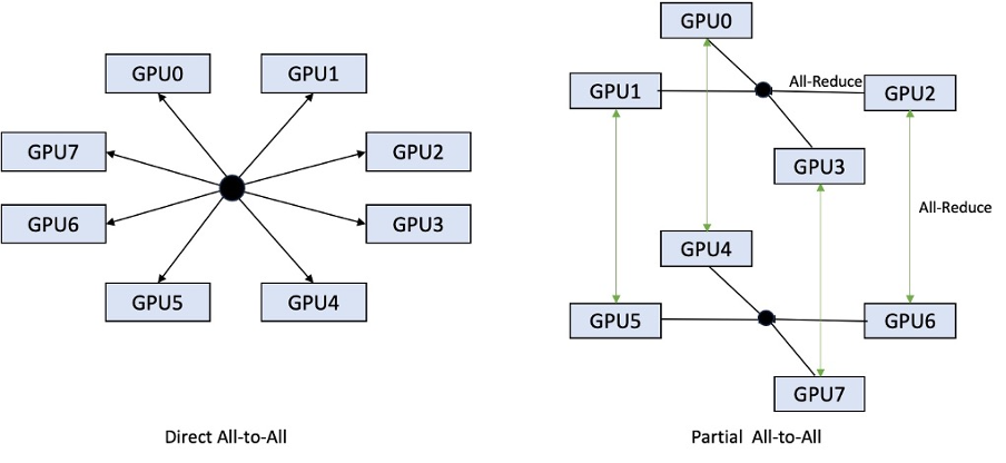
At AWS re:Invent 2023, LMI-Dist added new, optimized collective operations to speed up communication between GPUs, resulting in lower latency and higher throughput for models that are too big for a single GPU. These collectives are available exclusively for SageMaker, for p4d instances.

Whereas the previous iteration only supported sharding across all 8 GPUs, LMI 0.26.0 introduces support for a tensor parallel degree of 4, in a partial all-to-all pattern. This can be combined with SageMaker inference components, with which you can granularly configure how many accelerators should be allocated to each model deployed behind an endpoint. Together, these features provide better control over the resource utilization of the underlying instance, enabling you to increase model multi-tenancy by hosting different models behind one endpoint, or fine-tune the aggregate throughput of your deployment to match your model and traffic characteristics.

The following figure compares direct all-to-all with partial all-to-all.

TensorRT-LLM backend

NVIDIA’s TensorRT-LLM was introduced as part of the previous LMI DLC release (0.25.0), enabling state-of-the-art GPU performance and optimizations like SmoothQuant, FP8, and continuous batching for LLMs when using NVIDIA GPUs.

TensorRT-LLM requires models to be compiled into efficient engines before deployment. The LMI TensorRT-LLM DLC can automatically handle compiling a list of supported models just-in-time (JIT), before starting the server and loading the model for real-time inference. Version 0.26.0 of the DLC grows the list of supported models for JIT compilation, introducing Baichuan, ChatGLM , GPT2, GPT-J, InternLM, Mistral, Mixtral, Qwen, SantaCoder and StarCoder models.

JIT compilation adds several minutes of overhead to endpoint provisioning and scaling time, so it is always recommended to compile your model ahead-of-time. For a guide on how to do this and a list of supported models, see TensorRT-LLM ahead-of-time compilation of models tutorial. If your selected model isn’t supported yet, refer to TensorRT-LLM manual compilation of models tutorial to compile any other model that is supported by TensorRT-LLM.

Additionally, LMI now exposes native TensorRT-LLM SmootQuant quantization, with parameters to control alpha and scaling factor by token or channel. For more information about the related configurations, refer to TensorRT-LLM.

vLLM backend

The updated release of vLLM included in LMI DLC features performance improvements of up to 50% fueled by CUDA graph mode instead of eager mode. CUDA graphs accelerate GPU workloads by launching several GPU operations in one go instead of launching them individually, which reduces overheads. This is particularly effective for small models when using tensor parallelism.

The added performance comes at a trade-off of added GPU memory consumption. CUDA graph mode is now default for the vLLM backend, so if you are constrained on the amount of GPU memory available, you can set option.enforce_eager=True to force PyTorch eager mode.

Transformers-NeuronX backend

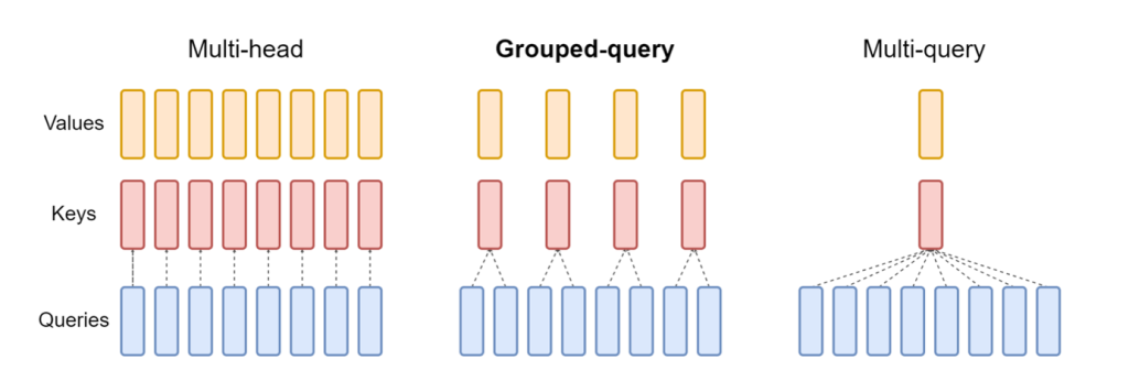
The updated release of NeuronX included in the LMI NeuronX DLC now supports models that feature the grouped-query attention mechanism, such as Mistral-7B and LLama2-70B. Grouped-query attention is an important optimization of the default transformer attention mechanism, where the model is trained with fewer key and value heads than query heads. This reduces the size of the KV cache on GPU memory, allowing for greater concurrency, and improving price-performance.

The following figure illustrates multi-head, grouped-query, and multi-query attention methods (source).

Different KV cache sharding strategies are available to suit different types of workloads. For more information on sharding strategies, see Grouped-query attention (GQA) support. You can enable your desired strategy (shard-over-heads, for example) with the following code:

option.group_query_attention=shard-over-heads

Additionally, the new implementation of NeuronX DLC introduces a cache API for TransformerNeuronX that enables access to the KV cache. It allows you to insert and remove KV cache rows from new requests while you’re handing batched inference. Before introducing this API, the KV cache was recomputed for any newly added requests. Compared to LMI V7 (0.25.0), we have improved latency by more than 33% with concurrent requests, and support much higher throughput.

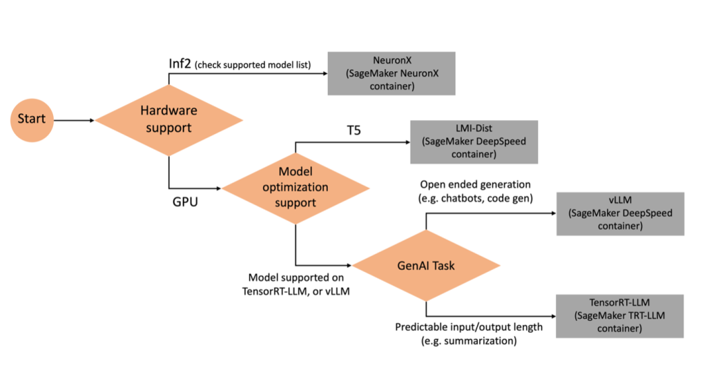
Selecting the right backend

To decide what backend to use based on the selected model and task, use the following flow chart. For individual backend user guides along with supported models, see LMI Backend User Guides.

Deploy Mixtral with LMI DLC with additional attributes

Let’s walk through how you can deploy the Mixtral-8x7B model with LMI 0.26.0 container and generate additional details like log_prob and finish_reason as part of the output. We also discuss how you can benefit from these additional attributes through a content generation use case.

The complete notebook with detailed instructions is available in the GitHub repo.

We start by importing the libraries and configuring the session environment:

import boto3
import sagemaker 
import json 
import io 
import numpy as np 
from sagemaker import Model, image_uris, serializers, deserializers 

role = sagemaker.get_execution_role() # execution role for the endpoint 
session = sagemaker.session.Session() # sagemaker session for interacting with different AWS APIs 
region = session._region_name # region name of the current SageMaker Studio environment

You can use SageMaker LMI containers to host models without any additional inference code. You can configure the model server either through the environment variables or a serving.properties file. Optionally, you could have a model.py file for any preprocessing or postprocessing and a requirements.txt file for any additional packages that are required to be installed.

In this case, we use the serving.properties file to configure the parameters and customize the LMI container behavior. For more details, refer to the GitHub repo. The repo explains details of the various configuration parameters that you can set. We need the following key parameters:

• engine – Specifies the runtime engine for DJL to use. This drives the sharding and the model loading strategy in the accelerators for the model.
• option.model_id – Specifies the Amazon Simple Storage Service (Amazon S3) URI of the pre-trained model or the model ID of a pretrained model hosted inside a model repository on Hugging Face. In this case, we provide the model ID for the Mixtral-8x7B model.
• option.tensor_parallel_degree – Sets the number of GPU devices over which Accelerate needs to partition the model. This parameter also controls the number of workers per model that will be started up when DJL serving runs. We set this value to max (maximum GPU on the current machine).
• option.rolling_batch – Enables continuous batching to optimize accelerator utilization and overall throughput. For the TensorRT-LLM container, we use auto.
• option.model_loading_timeout – Sets the timeout value for downloading and loading the model to serve inference.
• option.max_rolling_batch – Sets the maximum size of the continuous batch, defining how many sequences can be processed in parallel at any given time.

%%writefile serving.properties 
engine=MPI 
option.model_id=mistralai/Mixtral-8x7B-v0.1 
option.tensor_parallel_degree=max 
option.max_rolling_batch_size=32 
option.rolling_batch=auto 
option.model_loading_timeout = 7200

We package the serving.properties configuration file in the tar.gz format, so that it meets SageMaker hosting requirements. We configure the DJL LMI container with tensorrtllm as the backend engine. Additionally, we specify the latest version of the container (0.26.0).

image_uri = image_uris.retrieve(
   framework="djl-tensorrtllm",
   region=sess.boto_session.region_name,
   version="0.26.0"
)

Next, we upload the local tarball (containing the serving.properties configuration file) to an S3 prefix. We use the image URI for the DJL container and the Amazon S3 location to which the model serving artifacts tarball was uploaded, to create the SageMaker model object.

model = Model(image_uri=image_uri, model_data=code_artifact, role=role) 

instance_type = "ml.p4d.24xlarge" 
endpoint_name = sagemaker.utils.name_from_base("mixtral-lmi-model") 

model.deploy(
   initial_instance_count=1,
   instance_type=instance_type,
   endpoint_name=endpoint_name,
   container_startup_health_check_timeout=1800
)

As part of LMI 0.26.0, you can now use two additional fine-grained details about the generated output:

• log_probs – This is the log probability assigned by the model for each token in the streamed sequence chunk. You can use these as a rough estimate of model confidence by computing the joint probability of a sequence as the sum of the log probabilities of the individual tokens, which can be useful for scoring and ranking model outputs. Be mindful that LLM token probabilities are generally overconfident without calibration.
• finish_reason – This is the reason for generation completion, which can be reaching the maximum generation length, generating an EOS token, or generating a user-defined stop token. This is returned with the last streamed sequence chunk.

You can enable these by passing "details"=True as part of your input to the model.

Let’s see how you can generate these details. We use a content generation example to understand their application.

We define a LineIterator helper class, which has functions to lazily fetch bytes from a response stream, buffer them, and break down the buffer into lines. The idea is to serve bytes from the buffer while fetching more bytes from the stream asynchronously.

class LineIterator:
    def __init__(self, stream):
        # Iterator to get bytes from stream 
        self.byte_iterator = iter(stream)  
        # Buffer stream bytes until we get a full line
        self.buffer = io.BytesIO()  
        # Track current reading position within buffer
        self.read_pos = 0

   def __iter__(self):
        # Make class iterable 
        return self

    def __next__(self):
        while True:
           # Seek read position within buffer
           self.buffer.seek(self.read_pos)  
           # Try reading a line from current position
           line = self.buffer.readline()
           # If we have a full line
           if line and line[-1] == ord('n'):
               # Increment reading position past this line
               self.read_pos += len(line)  
               # Return the line read without newline char
               return line[:-1] 
           # Fetch next chunk from stream  
           try:
               chunk = next(self.byte_iterator)
           # Handle end of stream 
           except StopIteration:
               # Check if we have any bytes still unread
               if self.read_pos < self.buffer.getbuffer().nbytes:
                   continue
               # If not, raise StopIteration
               raise
           # Add fetched bytes to end of buffer
           self.buffer.seek(0, io.SEEK_END)  
           self.buffer.write(chunk['PayloadPart']['Bytes'])

Generate and use token probability as an additional detail

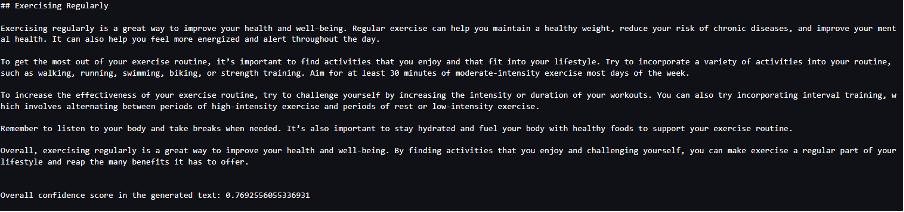
Consider a use case where we are generating content. Specifically, we’re tasked with writing a brief paragraph about the benefits of exercising regularly for a lifestyle-focused website. We want to generate content and output some indicative score of the confidence that the model has in the generated content.

We invoke the model endpoint with our prompt and capture the generated response. We set "details": True as a runtime parameter within the input to the model. Because the log probability is generated for each output token, we append the individual log probabilities to a list. We also capture the complete generated text from the response.

sm_client = boto3.client("sagemaker-runtime")

# Set details: True as a runtime parameter within the input.
body = {"inputs": prompt, "parameters": {"max_new_tokens":512, "details": True}}
resp = sm_client.invoke_endpoint_with_response_stream(EndpointName=endpoint_name, Body=json.dumps(body), ContentType="application/json")
event_stream = resp['Body']

overall_log_prob = []

for line in LineIterator(event_stream):
    resp = json.loads(line)
    if resp['token'].get('text') != None:
        token_log_prob = resp['token']['log_prob']
        overall_log_prob.append(token_log_prob)
    elif resp['generated_text'] != None:
        generated_text= resp['generated_text']

To calculate the overall confidence score, we calculate the mean of all the individual token probabilities and subsequently get the exponential value between 0 and 1. This is our inferred overall confidence score for the generated text, which in this case is a paragraph about the benefits of regular exercising.

print(generated_text) 
overall_score=np.exp(np.mean(overall_log_prob)) 
print(f"nnOverall confidence score in the generated text: {overall_score}")

This was one example of how you can generate and use log_prob, in the context of a content generation use case. Similarly, you can use log_prob as measure of confidence score for classification use cases.

Alternatively, you can use it for the overall output sequence or sentence-level scoring to evaluate the affect of parameters such as temperature on the generated output.

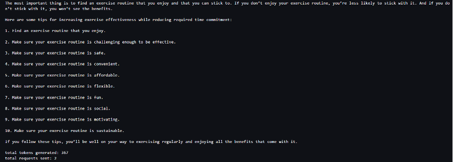
Generate and use finish reason as an additional detail

Let’s build on the same use case, but this time we’re tasked with writing a longer article. Additionally, we want to make sure that the output is not truncated due to generation length issues (max token length) or due to stop tokens being encountered.

To accomplish this, we use the finish_reason attribute generated in the output, monitor its value, and continue generating until the entire output is generated.

We define an inference function that takes a payload input and calls the SageMaker endpoint, streams back a response, and processes the response to extract generated text. The payload contains the prompt text as inputs and parameters like max tokens and details. The response is read in a stream and processed line by line to extract the generated text tokens into a list. We extract details like finish_reason. We call the inference function in a loop (chained requests) while adding more context each time, and track the number of tokens generated and number of requests sent until the model finishes.

def inference(payload):
    # Call SageMaker endpoint and get response stream
    resp = sm_client.invoke_endpoint_with_response_stream(EndpointName=endpoint_name, Body=json.dumps(payload), ContentType="application/json")
    event_stream = resp['Body']
    text_output = []
    for line in LineIterator(event_stream):
        resp = json.loads(line) 
        # Extract text tokens if present
        if resp['token'].get('text') != None:
            token = resp['token']['text']
            text_output.append(token)  
            print(token, end='')
        # Get finish reason if details present
        if resp.get('details') != None:
            finish_reason = resp['details']['finish_reason']
            # Return extracted output, finish reason and token length
            return payload['inputs'] + ''.join(text_output), finish_reason, len(text_output)

# set details: True as a runtime parameter within the input.
payload = {"inputs": prompt,  "parameters": {"max_new_tokens":256, "details": True}} 

finish_reason = "length"
# Print initial output 
print(f"Output: {payload['inputs']}", end='')  
total_tokens = 0
total_requests = 0
while finish_reason == 'length':
    # Call inference and get extracts
    output_text, finish_reason, out_token_len = inference(payload)
    # Update payload for next request
    payload['inputs'] = output_text 
    total_tokens += out_token_len
    total_requests += 1
# Print metrics
print(f"nntotal tokens generated: {total_tokens} ntotal requests sent: {total_requests}")

As we can see, even though the max_new_token parameter is set to 256, we use the finish_reason detail attribute as part of the output to chain multiple requests to the endpoint, until the entire output is generated.

Similarly, based on your use case, you can use stop_reason to detect insufficient output sequence length specified for a given task or unintended completion due to a human stop sequence.

Conclusion

In this post, we walked through the v0.26.0 release of the AWS LMI container. We highlighted key performance improvements, new model support, and new usability features. With these capabilities, you can better balance cost and performance characteristics while providing a better experience to your end-users.

To learn more about LMI DLC capabilities, refer to Model parallelism and large model inference. We’re excited to see how you use these new capabilities from SageMaker.

About the authors

João Moura is a Senior AI/ML Specialist Solutions Architect at AWS. João helps AWS customers – from small startups to large enterprises – train and deploy large models efficiently, and more broadly build ML platforms on AWS.

Rahul Sharma is a Senior Solutions Architect at AWS Data Lab, helping AWS customers design and build AI/ML solutions. Prior to joining AWS, Rahul has spent several years in the finance and insurance sector, helping customers build data and analytical platforms.

Qing Lan is a Software Development Engineer in AWS. He has been working on several challenging products in Amazon, including high performance ML inference solutions and high performance logging system. Qing’s team successfully launched the first Billion-parameter model in Amazon Advertising with very low latency required. Qing has in-depth knowledge on the infrastructure optimization and Deep Learning acceleration.

Jian Sheng is a Software Development Engineer at Amazon Web Services who has worked on several key aspects of machine learning systems. He has been a key contributor to the SageMaker Neo service, focusing on deep learning compilation and framework runtime optimization. Recently, he has directed his efforts and contributed to optimizing the machine learning system for large model inference.

Tyler Osterberg is a Software Development Engineer at AWS. He specializes in crafting high-performance machine learning inference experiences within SageMaker. Recently, his focus has been on optimizing the performance of Inferentia Deep Learning Containers on the SageMaker platform. Tyler excels in implementing performant hosting solutions for large language models and enhancing user experiences using cutting-edge technology.

Rupinder Grewal is a Senior AI/ML Specialist Solutions Architect with AWS. He currently focuses on serving of models and MLOps on Amazon SageMaker. Prior to this role, he worked as a Machine Learning Engineer building and hosting models. Outside of work, he enjoys playing tennis and biking on mountain trails.

Dhawal Patel is a Principal Machine Learning Architect at AWS. He has worked with organizations ranging from large enterprises to mid-sized startups on problems related to distributed computing, and Artificial Intelligence. He focuses on Deep learning including NLP and Computer Vision domains. He helps customers achieve high performance model inference on SageMaker.

Read More

Amazon Rekognition makes it easy to add image and video analysis to your applications. It’s based on the same proven, highly scalable, deep learning technology developed by Amazon’s computer vision scientists to analyze billions of images and videos daily. It requires no machine learning (ML) expertise to use and we’re continually adding new computer vision features to the service. Amazon Rekognition includes a simple, easy-to-use API that can quickly analyze any image or video file that’s stored in Amazon Simple Storage Service (Amazon S3).

Customers across industries such as advertising and marketing technology, gaming, media, and retail & e-commerce rely on images uploaded by their end-users (user-generated content or UGC) as a critical component to drive engagement on their platform. They use Amazon Rekognition content moderation to detect inappropriate, unwanted, and offensive content in order to protect their brand reputation and foster safe user communities.

In this post, we will discuss the following:

• Content Moderation model version 7.0 and capabilities
• How does Amazon Rekognition Bulk Analysis work for Content Moderation
• How to improve Content Moderation prediction with Bulk Analysis and Custom Moderation

Content Moderation Model Version 7.0 and Capabilities

Amazon Rekognition Content Moderation version 7.0 adds 26 new moderation labels and expands the moderation label taxonomy from a two-tier to a three-tier label category. These new labels and the expanded taxonomy enable customers to detect fine-grained concepts on the content they want to moderate. Additionally, the updated model introduces a new capability to identify two new content types, animated and illustrated content. This allows customers to create granular rules for including or excluding such content types from their moderation workflow. With these new updates, customers can moderate content in accordance with their content policy with higher accuracy.

Let’s look at a moderation label detection example for the following image.

The following table shows the moderation labels, content type, and confidence scores returned in the API response.

To obtain the full taxonomy for Content Moderation version 7.0, visit our developer guide.

Bulk Analysis for Content Moderation

Amazon Rekognition Content Moderation also provides batch image moderation in addition to real-time moderation using Amazon Rekognition Bulk Analysis. It enables you to analyze large image collections asynchronously to detect inappropriate content and gain insights into the moderation categories assigned to the images. It also eliminates the need for building a batch image moderation solution for customers.

You can access the bulk analysis feature either via the Amazon Rekognition console or by calling the APIs directly using the AWS CLI and the AWS SDKs. On the Amazon Rekognition console, you can upload the images you want to analyze and get results with a few clicks. Once the bulk analysis job completes, you can identify and view the moderation label predictions, such as Explicit, Non-Explicit Nudity of Intimate parts and Kissing, Violence, Drugs & Tobacco, and more. You also receive a confidence score for each label category.

Create a bulk analysis job on the Amazon Rekognition console

Complete the following steps to try Amazon Rekognition Bulk Analysis:

1. On the Amazon Rekognition console, choose Bulk Analysis in the navigation pane.
2. Choose Start Bulk Analysis.
3. Enter a job name and specify the images to analyze, either by entering an S3 bucket location or by uploading images from your computer.
4. Optionally, you can select an adapter to analyze images using the custom adapter that you have trained using Custom Moderation.
5. Choose Start analysis to run the job.
   

When the process is complete, you can see the results on the Amazon Rekognition console. Also, a JSON copy of the analysis results will be stored in the Amazon S3 output location.

Amazon Rekognition Bulk Analysis API request

In this section, we guide you through creating a bulk analysis job for image moderation using programming interfaces. If your image files aren’t already in an S3 bucket, upload them to ensure access by Amazon Rekognition. Similar to creating a bulk analysis job on the Amazon Rekognition console, when invoking the StartMediaAnalysisJob API, you need to provide the following parameters:

• OperationsConfig – These are the configuration options for the media analysis job to be created:
  • MinConfidence – The minimum confidence level with the valid range of 0–100 for the moderation labels to return. Amazon Rekognition doesn’t return any labels with a confidence level lower than this specified value.
• Input – This includes the following:
  • S3Object – The S3 object information for the input manifest file, including the bucket and name of the file. input file includes JSON lines for each image stored on S3 bucket. for example: {"source-ref": "s3://MY-INPUT-BUCKET/1.jpg"}
• OutputConfig – This includes the following:
  • S3Bucket – The S3 bucket name for the output files.
  • S3KeyPrefix – The key prefix for the output files.

See the following code:

import boto3
import os
import datetime
import time
import json
import uuid

region = boto3.session.Session().region_name
s3=boto3.client('s3')
rekognition_client=boto3.client('rekognition', region_name=region)

min_confidence = 50
input_bucket = "MY-INPUT-BUCKET"

input_file = "input_file.jsonl"
output_bucket = "MY-OUTPUT-BUCKET"
key_prefix = "moderation-results"
job_name = "bulk-analysis-demo"

job_start_response = rekognition_client.start_media_analysis_job(
    OperationsConfig={"DetectModerationLabels": {"MinConfidence": min_confidence}},
    JobName = job_name,
    Input={"S3Object": {"Bucket": input_bucket, "Name": input_file}},
    OutputConfig={"S3Bucket": output_bucket, "S3KeyPrefix": key_prefix},
)

job_id = job_start_response["JobId"]
max_tries = 60
while max_tries > 0:
    max_tries -= 1
    job = rekognition_client.get_media_analysis_job(JobId=job_id)
    job_status = job["Status"]
    if job_status in ["SUCCEEDED", "FAILED"]:
        print(f"Job {job_name} is {job_status}.")
        if job_status == "SUCCEEDED":
            print(
                f"Bulk Analysis output file copied to:n"
                f"tBucket: {job['Results']['S3Object']['Bucket']}n"
                f"tObject: {job['Results']['S3Object']['Name']}."
            )
        break
    else:
        print(f"Waiting for {job_name}. Current status is {job_status}.")
    time.sleep(10)

You can invoke the same media analysis using the following AWS CLI command:

aws rekognition start-media-analysis-job 
--operations-config "DetectModerationLabels={MinConfidence='50'}" 
--input "S3Object={Bucket=input_bucket,Name=input_file.jsonl}" 
--output-config "S3Bucket=output_bucket,S3KeyPrefix=moderation-results"

Amazon Rekognition Bulk Analysis API results

To get a list of bulk analysis jobs, you can use ListMediaAnalysisJobs. The response includes all the details about the analysis job input and output files and the status of the job:

# get the latest 10 media analysis jobs
moderation_job_list = rekognition_client.list_media_analysis_jobs(MaxResults=10, NextToken="")
for job_result in moderation_job_list["MediaAnalysisJobs"]:
 print(f'JobId: {job_result["JobId"]} ,Status: {job_result["Status"]},n
Summary: {job_result["ManifestSummary"]["S3Object"]["Name"]}, n
Result: {job_result["Results"]["S3Object"]["Name"]}n')

You can also invoke the list-media-analysis-jobs command via the AWS CLI:

aws rekognition list-media-analysis-jobs --max-results 10

Amazon Rekognition Bulk Analysis generates two output files in the output bucket. The first file is manifest-summary.json, which includes bulk analysis job statistics and a list of errors:

{
    "version": "1.0",
    "statistics": {
      "total-json-lines": 2,
      "valid-json-lines": 2,
      "invalid-json-lines": 0
    },
    "errors": []
 }

The second file is results.json, which includes one JSON line per each analyzed image in the following format. Each result includes the top-level category (L1) of a detected label and the second-level category of the label (L2), with a confidence score between 1–100. Some Taxonomy Level 2 labels may have Taxonomy Level 3 labels (L3). This allows a hierarchical classification of the content.

{
  "source-ref": "s3://MY-INPUT-BUCKET/1.jpg",
    "detect-moderation-labels": {
    "ModerationLabels": [
      {
        "ParentName": "Products",
        "TaxonomyLevel": 3,
        "Confidence": 91.9385,
        "Name": "Pills"
      },
      {
        "ParentName": "Drugs & Tobacco",
        "TaxonomyLevel": 2,
        "Confidence": 91.9385,
        "Name": "Products"
      },
      {
        "ParentName": "",
        "TaxonomyLevel": 1,
        "Confidence": 91.9385,
        "Name": "Drugs & Tobacco"
      }
    ],
    "ModerationModelVersion": "7.0",
    "ContentTypes": [
      
    ]
  }
}

You can use Custom Moderation adapters later to analyze your images by simply selecting the custom adapter while creating a new bulk analysis job or via API by passing the custom adapter’s unique adapter ID.

Summary

In this post, we provided an overview of Content Moderation version 7.0, Bulk Analysis for Content Moderation, and how to improve Content Moderation predictions using Bulk Analysis and Custom Moderation. To try the new moderation labels and bulk analysis, log in to your AWS account and check out the Amazon Rekognition console for Image Moderation and Bulk Analysis.

About the authors

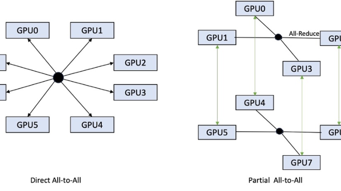
Mehdy Haghy is a Senior Solutions Architect at AWS WWCS team, specializing in AI and ML on AWS. He works with enterprise customers, helping them migrate, modernize, and optimize their workloads for the AWS cloud. In his spare time, he enjoys cooking Persian foods and electronics tinkering.

Shipra Kanoria is a Principal Product Manager at AWS. She is passionate about helping customers solve their most complex problems with the power of machine learning and artificial intelligence. Before joining AWS, Shipra spent over 4 years at Amazon Alexa, where she launched many productivity-related features on the Alexa voice assistant.

Maria Handoko is a Senior Product Manager at AWS. She focuses on helping customers solve their business challenges through machine learning and computer vision. In her spare time, she enjoys hiking, listening to podcasts, and exploring different cuisines.

Read More