Robotic Transformer 2 (RT-2) is a novel vision-language-action (VLA) model that learns from both web and robotics data, and translates this knowledge into generalised instructions for robotic control.Read More
Robotic Transformer 2 (RT-2) is a novel vision-language-action (VLA) model that learns from both web and robotics data, and translates this knowledge into generalised instructions for robotic control.Read More

Robotic Transformer 2 (RT-2) is a novel vision-language-action (VLA) model that learns from both web and robotics data, and translates this knowledge into generalised instructions for robotic control.Read More
Robotic Transformer 2 (RT-2) is a novel vision-language-action (VLA) model that learns from both web and robotics data, and translates this knowledge into generalised instructions for robotic control.Read More

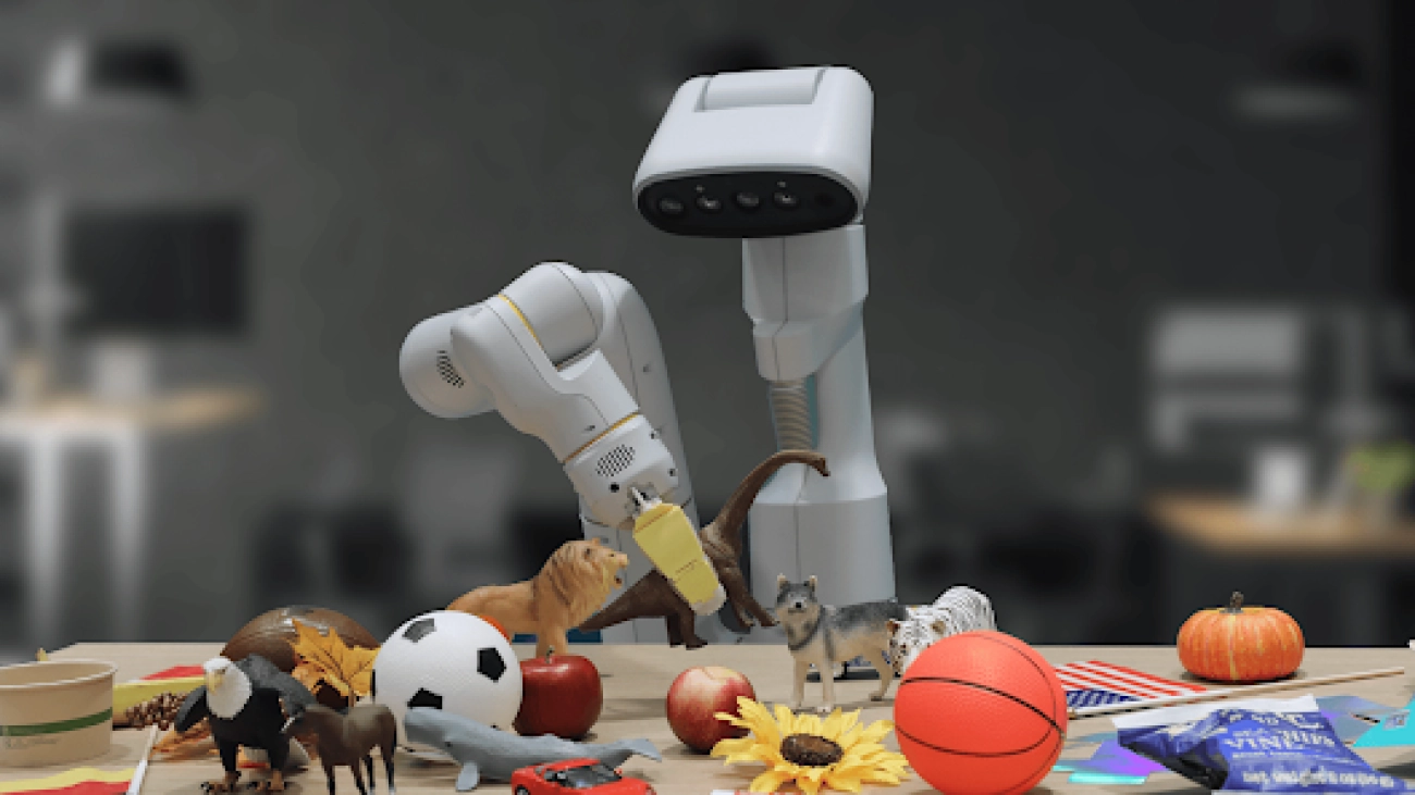
Introducing Robotic Transformer 2 (RT-2), a novel vision-language-action (VLA) model that learns from both web and robotics data, and translates this knowledge into generalised instructions for robotic control, while retaining web-scale capabilities. This work builds upon Robotic Transformer 1 (RT-1), a model trained on multi-task demonstrations which can learn combinations of tasks and objects seen in the robotic data. RT-2 shows improved generalisation capabilities and semantic and visual understanding, beyond the robotic data it was exposed to. This includes interpreting new commands and responding to user commands by performing rudimentary reasoning, such as reasoning about object categories or high-level descriptions. Read More
From smart factories to next-generation railway systems, developers and enterprises across the world are racing to fuel industrial digitalization opportunities at every scale.
Key to this is the open-source Universal Scene Description (USD) framework, or OpenUSD, along with metaverse applications powered by AI.
OpenUSD, originally developed by Pixar for large-scale feature film pipelines for animation and visual effects, offers a powerful engine for high-fidelity 3D worlds, as well as an expansive ecosystem for the era of AI and the metaverse. Across automotive, healthcare, manufacturing and other industries, businesses are adopting OpenUSD for various applications.
Developers can use the extensibility of OpenUSD to integrate the latest AI tools, as well as top digital content-creation solutions, into their custom 3D workflows and applications.
At enterprises like BMW Group, in-house developers are building custom applications to optimize and interact with their digital twin use cases. The automaker developed an application that allows factory planners to collaborate in real time on virtual factories using NVIDIA Omniverse, an OpenUSD development platform for building and connecting 3D tools.
Startups like Move.ai, SmartCow and ipolog are also developing groundbreaking metaverse technologies with OpenUSD. Using USD in Omniverse’s modular development platform allows startups and small businesses to easily launch new tools in the metaverse for larger enterprises to use.
In addition, leading 3D solution providers, including Esri, Bentley Systems and Vectorworks, are connecting their technologies with OpenUSD to enable new capabilities in the metaverse and reach more customers. Building on OpenUSD ensures their applications can be continuously expanded to meet the industrial metaverse’s evolving needs.
“USD helps us provide customers with even more flexibility in the 3D design process,” said Dave Donley, senior director of rendering and research at Vectorworks. “By embracing USD, Vectorworks and its users are poised to lead the charge toward a more collaborative and innovative future in industries such as architecture, landscape design and entertainment.”
Linear and siloed workflows used to be the norm in 3D content creation. Today, enterprises must integrate their diverse, distributed, highly skilled teams and expand their offerings to remain competitive — most notably in generative AI.
Fluid design collaboration is critical for this, as is the ability for developers to work in open, modular and extensible frameworks. As the pace of AI and metaverse innovation increases, businesses attempting to build new features and capabilities in closed environments are likely to lag behind.
The 3D worlds of the metaverse — which are ushering in a new era of design, simulation and AI advancements — require a common framework to enable scalability and interconnection. As with the 2D web, the success of the metaverse will depend on its interoperability as governed by open standards and protocols.
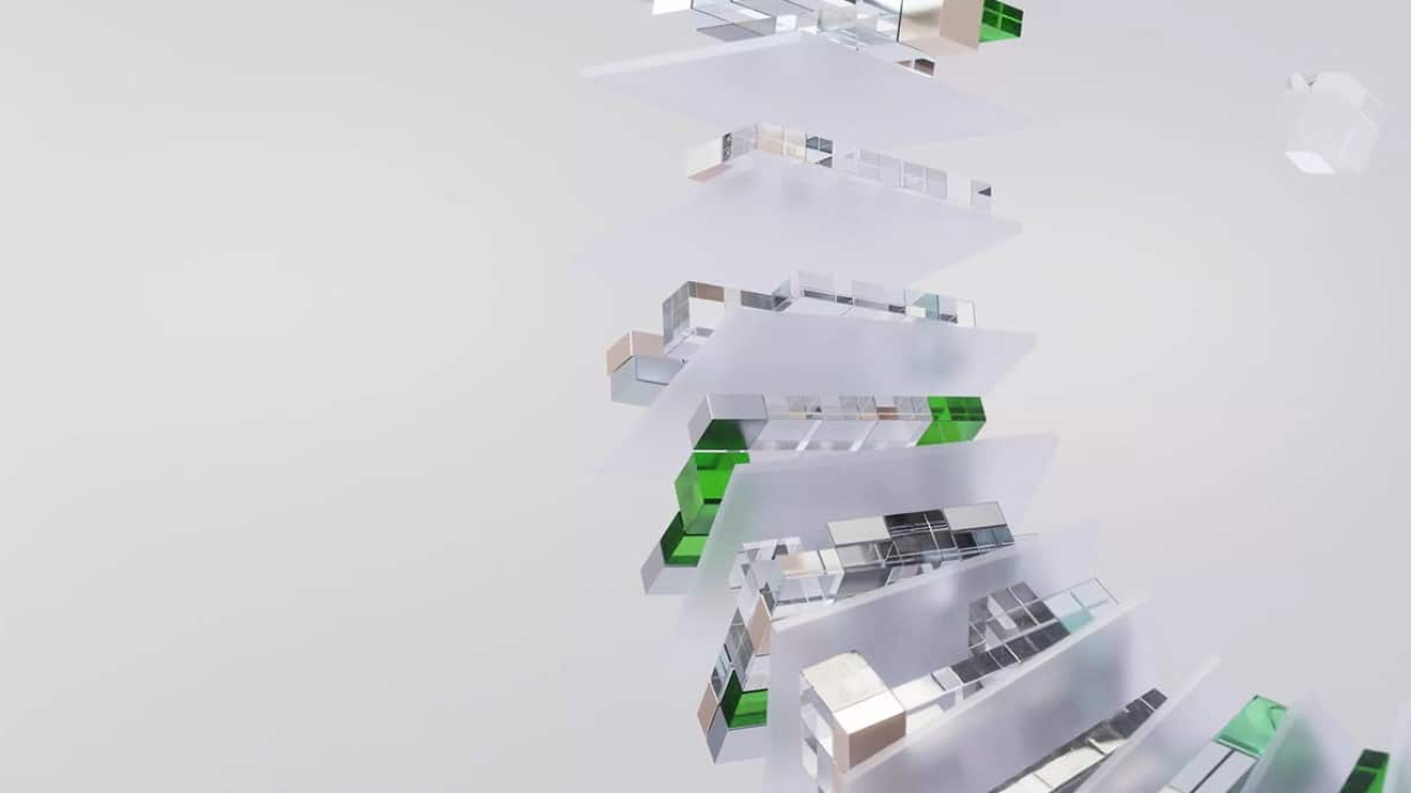
OpenUSD is well-suited for diverse metaverse applications due to its extensibility and ability to support a wide variety of properties for defining and rendering objects. More than just a file format, the interchange framework connects a robust ecosystem of creative and developer tools.
Cesium, a platform for 3D geospatial workflows, uses USD to enable enterprises building industrial metaverse applications in construction, robotics, simulation and digital twins for climate change.
“Leveraging the interoperability of USD with 3D Tiles and glTF, we create additional workflows, like importing content from Bentley LumenRT, Trimble Sketchup, Autodesk Revit, Autodesk 3ds Max and Esri ArcGIS CityEngine into NVIDIA Omniverse in precise 3D geospatial context,” said Shehzan Mohammed, director of 3D engineering and ecosystems at Cesium.
3D tools interoperate seamlessly with OpenUSD, allowing users to work efficiently across various tools and pipelines. USD’s efficient referencing and layering allows teams to non-destructively edit projects in real time and preserve all source content, enabling iterative, collaborative workflows. Designed to handle large-scale scenes with millions of assets and complex datasets, OpenUSD is ideal for developers building applications to support virtual worlds.
Learn more about the unique capabilities of USD in the video below, as well as in the article, “What You Need to Know About Universal Scene Description.”
NVIDIA Omniverse interconnects diverse 3D tools and datasets with OpenUSD to unlock new possibilities for large-scale, physically accurate virtual worlds and industrial digitalization applications.
Built for developers by developers, Omniverse is open and highly modular. Omniverse Code and Kit enable developers to build advanced, real-time simulation solutions for industrial digitalization and perception AI. They can use all of the platform’s key components, such as Omniverse Nucleus and RTX Renderer, and core technologies to develop solutions designed for their customer needs.
People of all experience levels can build with OpenUSD on Omniverse. Beginners can develop tools with little to no code using existing platform extensions. Experienced developers can use templates or build from scratch with Python or C++ to produce their own powerful apps and extensions — as well as combine them with existing ones to create tools customized for their needs. In addition, visual programming tools like OmniGraph make it easy to set up and perform advanced procedural tasks with just a few clicks.
For example, a warehouse simulation tool can be developed by combining extensions for building layout, warehouse objects, smart object placement and user interfaces that can be fine-tuned for specific needs.
Plus, Omniverse foundation applications like USD Composer and USD Presenter are modular, so users can work with just the functionality they need, and add their own code or extensions to customize apps for different workflows. Developers can easily access and tap into the Python source code of Omniverse extensions in Omniverse Kit.
Learn about the latest advancements in design, simulation and AI by joining NVIDIA at SIGGRAPH, a computer graphics conference running Aug. 6-10. NVIDIA founder and CEO Jensen Huang will deliver a keynote address on Tuesday, Aug. 8, at 8 a.m. PT.
Join NVIDIA for OpenUSD day at SIGGRAPH on Wednesday, Aug. 9, starting at 9 a.m. PT, for a full day of presentations about the framework’s latest developments. NVIDIA will also present award-winning research on rendering and generative AI, as well as host various sessions and hands-on labs for attendees to experience the latest developments in OpenUSD, graphics and more.
Get started with NVIDIA Omniverse by downloading the standard license free, or learn how Omniverse Enterprise can connect your team. Developers can check out these Omniverse resources to begin building on the platform.
Stay up to date on the platform by subscribing to the newsletter and following NVIDIA Omniverse on Instagram, LinkedIn, Medium, Threads and Twitter. For more, check out our forums, Discord server, Twitch and YouTube channels.
Determining on the fly how much additional audio to process to resolve ambiguities increases accuracy while reducing latency relative to fixed-lookahead approaches.Read More
For our midyear update, we’d like to share three of our best practices based on this guidance and what we’ve done in our pre-launch design, reviews and development of ge…Read More
This research paper was presented at the 17th USENIX Symposium on Operating Systems Design and Implementation (OSDI), a premier forum for discussing the design, implementation, and implications of systems software.
Cloud platforms aim to provide a seamless user experience, alleviating the challenge and complexity of managing physical servers in datacenters. Hardware failures are one such challenge, as individual server components can fail independently, and while failures affecting individual customers are rare, cloud platforms encounter a substantial volume of server failures. Currently, when a single component in a server fails, the entire server needs to be serviced by a technician. This all-or-nothing operating model is increasingly becoming a hindrance to achieving cloud sustainability goals.
A sustainable cloud platform should be water-positive and carbon-negative. Water consumption in datacenters primarily arises from the need for cooling, and liquid cooling has emerged as a potential solution for waterless cooling. Paradoxically, liquid cooling also increases the complexity and time required to repair servers. Therefore, reducing the demand for repairs becomes essential to achieving water-positive status.
To become carbon-negative, Microsoft has been procuring renewable energy for its datacenters since 2016. Currently, Azure’s carbon emissions largely arise during server manufacturing, as indicated in Microsoft’s carbon emission report. Extending the lifetime of servers, which Microsoft has recently done to a minimum of six years, is a key strategy to reduce server-related carbon emissions. However, longer server lifetimes highlight the importance of server repairs, which not only contribute significantly to costs but also to carbon emissions. Moreover, sourcing replacement components can sometimes pose challenges. Consequently, finding ways to minimize the need for repairs becomes crucial.
Spotlight: On-Demand EVENT
On-Demand
Watch now to learn about some of the most pressing questions facing our research community and listen in on conversations with 120+ researchers around how to ensure new technologies have the broadest possible benefit for humanity.
To support Microsoft sustainability goals, our paper, “Hyrax: Fail-in-Place Server Operation in Cloud,” proposes that cloud platforms adopt a fail-in-place paradigm where servers with faulty components continue to host virtual machines (VMs) without the need for immediate repairs. With this approach, cloud platforms could significantly reduce repair requirements, decreasing costs and carbon emissions at the same time. However, implementing fail-in-place in practice poses several challenges.
First, we want to ensure graceful degradation, where faulty components are identified and deactivated in a controlled manner. Second, deactivating common components like dual in-line memory modules (DIMMs) can significantly impact server performance due to reduced memory interleaving. It is crucial to prevent VM customers from experiencing loss in performance resulting from these deactivations. Finally, the cloud platform must be capable of using the capacity of servers with deactivated components, necessitating algorithmic changes in VM scheduling and structural adjustments in the cloud control plane.
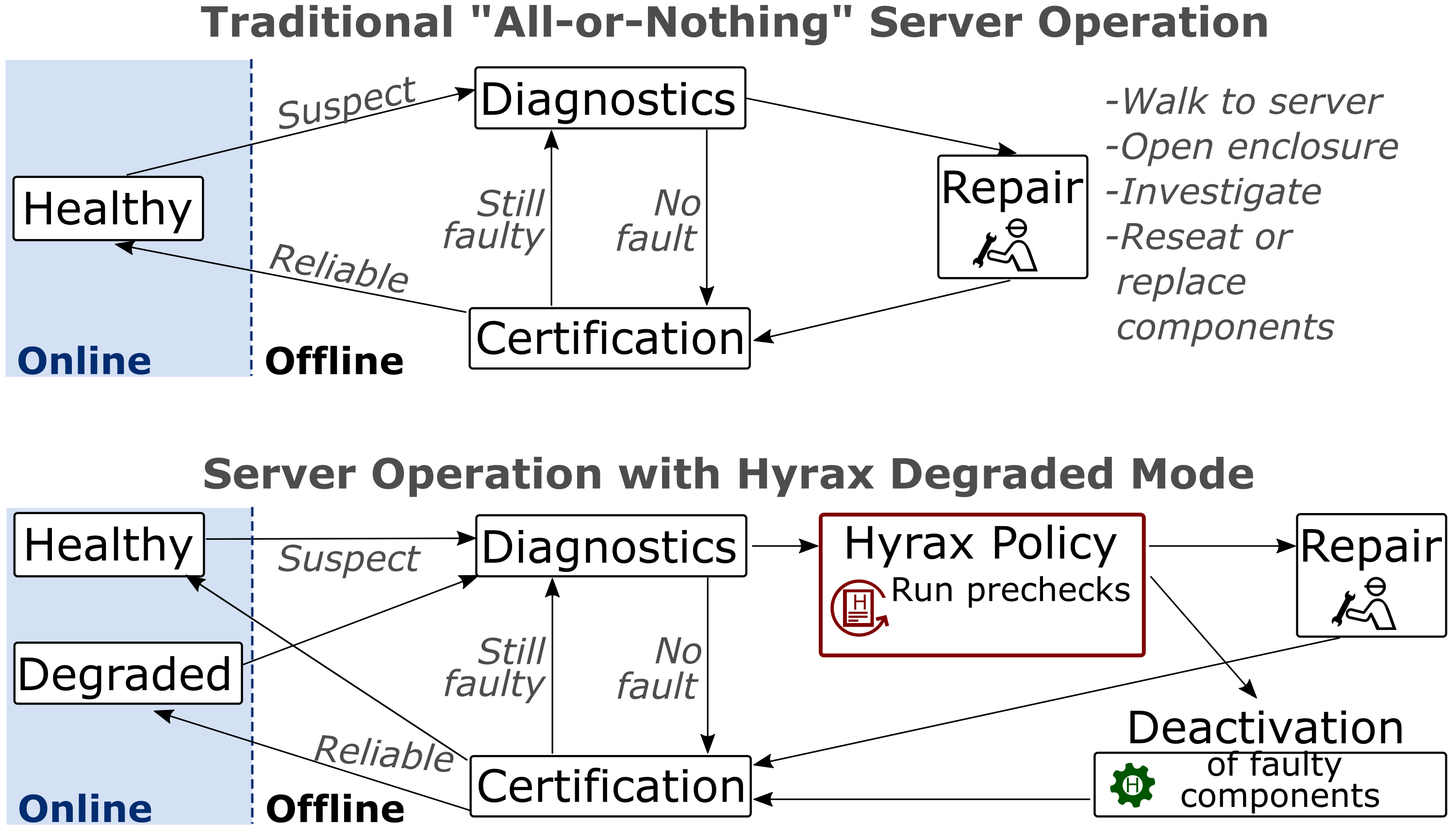
To address these challenges, our paper introduces Hyrax, the first implementation of fail-in-place for cloud compute servers. Through a multi-year study of component failures across five server generations, we found that existing servers possess sufficient redundancy to overcome the most common types of server component failures. We propose effective mechanisms for component deactivation that can mitigate a wide range of possibilities, including issues like corroded connectors or chip failures. Additionally, Hyrax introduces a degraded server state and scheduling optimizations to the production control plane, enabling effective utilization of servers with deactivated components, as illustrated in Figure 1.
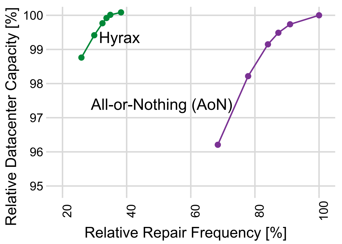
Our results demonstrate that Hyrax achieves a 60 percent reduction in repair demand without compromising datacenter capacity, as shown in Figure 2. This reduction in repairs leads to a 5 percent decrease in embodied carbon emissions over a typical six-year deployment period, as fewer replacement components are needed. In a subsequent study, we show that Hyrax enables servers to run for 30 percent longer, resulting in a proportional reduction in embodied carbon. We also demonstrate that Hyrax does not impact VM performance.
One of Hyrax’s key technical challenges is the need to deactivate components at the firmware level, as software-based deactivations prove to be insufficient. This requirement requires addressing previously unexplored performance implications.
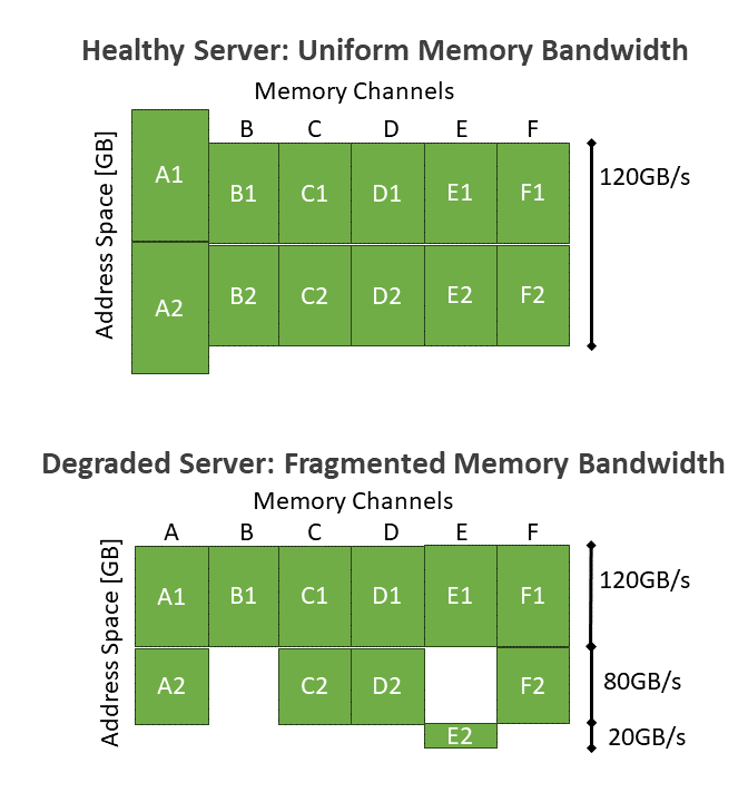
A good example is the deactivation of a memory module, specifically a DIMM. To understand DIMM deactivation, it is important to consider how CPUs access memory, which is usually hidden from software. This occurs at the granularity of a cache line, which is 64 bytes and resides on a single DIMM. Larger data is divided into cache lines and distributed among all DIMMs connected to a CPU in a round-robin fashion. This interleaving mechanism ensures that while one DIMM is handling cache line N, another DIMM serves cache line N+1. From a software standpoint, memory is typically presented as a uniform address space that encompasses all cache lines across all the DIMMs attached to the CPU. Accessing any portion of this address space is equally fast in terms of memory bandwidth. Figure 3 shows an example of a server with six memory channels populated with two 32-GB DIMMs each. From the software perspective, the entire 384 GB of address space appears indistinguishable and offers a consistent 120 GB/sec bandwidth.
However, deactivating a DIMM causes the interleaving policy to reconfigure in unexpected ways. Figure 3 demonstrates this scenario, where the second DIMM on channel B (B2) has been identified as faulty and subsequently deactivated. Consequently, three different parts of the address space exhibit different characteristics: 120 GB/sec (six-way interleaving), 80 GB/sec (four-way interleaving), and 20 GB/sec (one-way interleaving). These performance differences are invisible to software and naively scheduling VMs on such a server can lead to variable performance, a suboptimal outcome.
Hyrax enables cloud platforms to work around this issue by scheduling VMs on only the parts of the address space that offer sufficient performance for that VM’s requirements. Our paper discusses how this works in more detail.
Hyrax is the first fail-in-place system for cloud computing servers, paving the way for future improvements. One potential enhancement involves reconsidering the approach to memory regions with 20 GB/sec memory bandwidth. Instead of using them only for small VMs, we could potentially allocate these regions to accommodate large data structures, such as by adding buffers for input-output devices that require more than 20 GB/sec of bandwidth.
Failing-in-place offers significant flexibility when it comes to repairs. For example, instead of conducting daily repair trips to individual servers scattered throughout a datacenter, we are exploring the concept of batching repairs, where technicians would visit a row of server racks once every few weeks to address issues across multiple servers simultaneously. By doing so, we can save valuable time and resources while creating new research avenues for optimizing repair schedules that intelligently balance capacity loss and repair efforts.
Achieving sustainability goals demands collective efforts across society. In this context, we introduce fail-in-place as a research direction for both datacenter hardware and software systems, directly tied to water and carbon efficiency. Beyond refining the fail-in-place concept itself and exploring new server designs, this new paradigm also opens up new pathways for improving maintenance processes using an environmentally friendly approach.
The post A fail-in-place approach for sustainable server operations appeared first on Microsoft Research.
AI is improving ways to power the world by tapping the sun and the wind, along with cutting-edge technologies.
The latest episode in the I AM AI video series showcases how artificial intelligence can help optimize solar and wind farms, simulate climate and weather, enhance power grid reliability and resilience, advance carbon capture and power fusion breakthroughs.
It’s all enabled by NVIDIA and its energy-conscious partners, as they use and develop technology breakthroughs for a cleaner, safer, more sustainable future.
Homes and businesses need access to reliable, affordable fuel and electricity to power day-to-day activities.
Renewable energy sources — such as sunlight, wind and water — are scaling in deployments and available capacity. But they also burden legacy power grids built for traditional one-way power flow: from generation plants through transmission and distribution lines to end customers.
The latest advancements in AI and accelerated computing enable energy companies and utilities to balance power supply and demand in real time and manage distributed energy resources, all while lowering monthly bills to consumers.
The enterprises and startups featured in the new I AM AI video, and below, are using such innovations for a variety of clean energy use cases.
Companies are turning to AI to improve maintenance of renewable power-generation sites.
For example, reality capture platform DroneDeploy is using AI to evaluate solar farm layouts, maximize energy generated per site and automatically monitor the health of solar panels and other equipment in the field.
Renewable energy company Siemens Gamesa is working with NVIDIA to apply AI surrogate models to optimize its offshore wind farms to output maximum power at minimal cost. Together, the companies are exploring neural super resolution powered by the NVIDIA Omniverse and NVIDIA Modulus platforms to accelerate high-resolution wake simulation by 4,000x compared with traditional methods–from 40 days to just 15 minutes.
Italy-based THE EDGE COMPANY, a member of the NVIDIA Metropolis vision AI partner ecosystem, is tracking endangered birds near offshore wind farms to provide operators with real-time suggestions that can help prevent collisions and protect the at-risk species.
Energy grids also benefit from AI, which can help keep their infrastructure safe and efficient.
NVIDIA Metropolis partner Noteworthy AI deployed smart cameras powered by the NVIDIA Jetson platform for edge AI and robotics on Ohio-based utility FirstEnergy’s field trucks. Along with AI-enhanced computer vision, the cameras automate manual inspections of millions of power lines, poles and mounted devices.
Orbital Sidekick, a member of the NVIDIA Inception program for cutting-edge startups, has used hyperspectral imagery and edge AI to detect hundreds of suspected gas and hydrocarbon leaks across the globe. This protects worker health and safety while preventing costly accidents.
And Sweden-based startup Eneryield is using AI to detect signal anomalies in undersea cables, predict equipment failures to avoid costly repairs and enhance reliability of generated power.
AI and digital twins are unleashing a new wave of climate research, offering accurate, physics-informed weather modeling, high-resolution simulations of Earth and more.
NVIDIA Inception member Open Climate Fix built transformer-based AI models trained on terabytes of satellite data. Through granular, near-term forecasts of sunny and cloudy conditions over the U.K.’s solar panels, the nonprofit product lab has improved predictions of solar-energy generation by 3x. This reduces electricity produced using fossil fuels and helps decarbonize the country’s grid.
Plus, a team of researchers from the California Institute of Technology, Stanford University, and NVIDIA developed a neural operator architecture called Nested FNO to simulate pressure levels during carbon storage in a fraction of a second while doubling accuracy on certain tasks. This can help industries decarbonize and achieve emission-reduction goals.
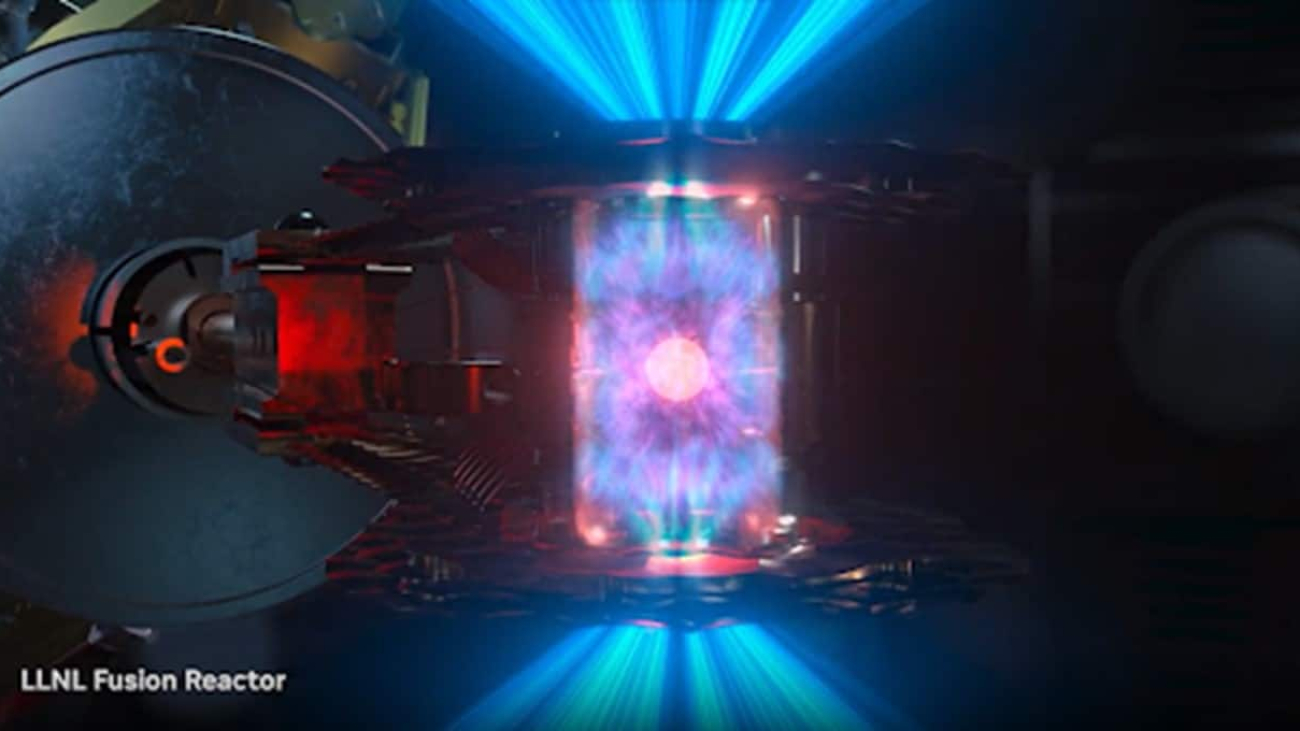
And Lawrence Livermore National Laboratory demonstrated the first successful application of nuclear fusion — considered the holy grail of clean energy — and used AI to simulate experimental results.
Learn more about AI for autonomous operations and grid modernization in energy.
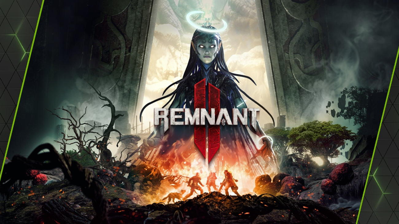
Get ready for Gunfire Games and Gearbox Publishing’s highly anticipated Remnant II, available for members to stream on GeForce NOW at launch. It leads eight new games coming to the cloud gaming platform.
Ultimate and Priority members, make sure to grab the Guild Wars 2 rewards, available now through Thursday, Aug. 31. Visit the GeForce NOW Rewards portal and opt in to rewards.

Kick off the weekend with one of the hottest new games in the cloud. Remnant II from Gunfire Games and Gearbox Publishing, sequel to the hit game Remnant: From the Ashes, is newly launched in the cloud for members to stream.
Go head to head against new deadly creatures and god-like bosses while exploring terrifying new worlds with different types of creatures, weapons and items. With various stories woven throughout, each playthrough will be different from the last, making each experience unique for endless replayability.
Find secrets and unlock different Archetypes, each with their own special set of abilities. Members can brave it alone or team up with buddies to explore the depths of the unknown and stop an evil from destroying reality itself. Just remember — friendly fire is on, so pick your squad wisely.
Upgrade to an Ultimate membership to play Remnant II and more than 1,600 titles at RTX 4080 quality, with support for 4K 120 frames per second gameplay and ultrawide resolutions. Ultimate and Priority members can also experience higher frame rates with DLSS technology for AI-powered graphics on their RTX-powered cloud gaming rigs.
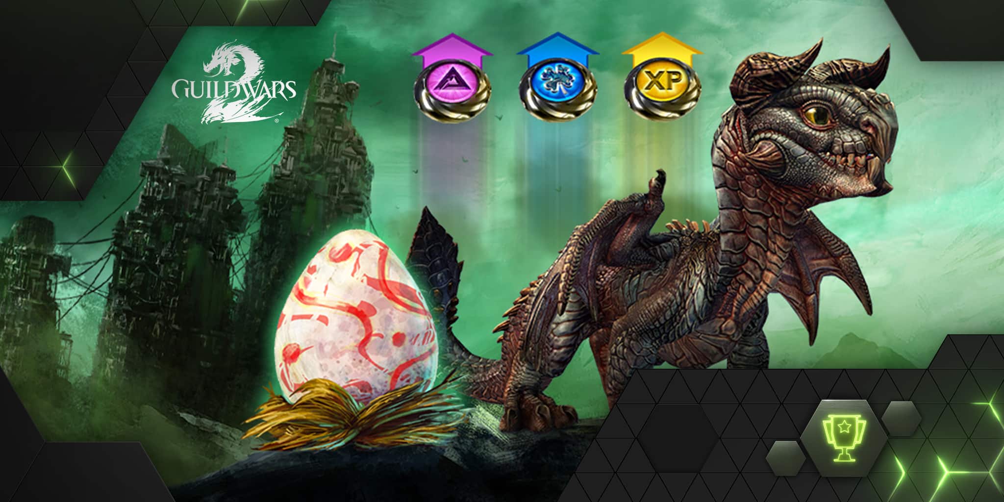
Ultimate and Priority members can now grab their free, exclusive rewards for Guild Wars 2, featuring the “Always Prepared” and “Booster” bundles, available through the end of August.
The “Always Prepared” bundle includes ten Transmutation Charges to change character appearance, a Revive Orb that returns a player to 50% health at their current location and a top hat to add style to the character. On top of that, the “Booster” bundle includes an Item Booster, Karma Booster, Experience Booster, a 10-Slot Bag and a Black Lion Miniature Claim Ticket, which can be exchanged in game for a mini-pet of choice.
Visit the GeForce NOW Rewards portal to update the settings to receive special offers and in-game goodies. Better hurry — these rewards are available for a limited time on a first-come, first-served basis.
Grab them in time for the fourth expansion of Guild Wars 2, coming to GeForce NOW at launch on Tuesday, Aug. 22. The “Secrets of the Obscure” paid expansion includes a new storyline, powerful combat options, new mount abilities and more.

Remnant II is one of the eight games available this week on GeForce NOW. Check out the complete list of new games:
What are you planning to play this weekend? Let us know on Twitter or in the comments below.
It’s up to you to save humanity from the Root. Which Archetype are you choosing:
Challenger
Medic
Gunslinger
Handler
Hunter
—
NVIDIA GeForce NOW (@NVIDIAGFN) July 26, 2023