We’re forming a new industry body to promote the safe and responsible development of frontier AI systems: advancing AI safety research, identifying best practices and standards, and facilitating information sharing among policymakers and industry.OpenAI Blog

AWS Reaffirms its Commitment to Responsible Generative AI
As a pioneer in artificial intelligence and machine learning, AWS is committed to developing and deploying generative AI responsibly
As one of the most transformational innovations of our time, generative AI continues to capture the world’s imagination, and we remain as committed as ever to harnessing it responsibly. With a team of dedicated responsible AI experts, complemented by our engineering and development organization, we continually test and assess our products and services to define, measure, and mitigate concerns about accuracy, fairness, intellectual property, appropriate use, toxicity, and privacy. And while we don’t have all of the answers today, we are working alongside others to develop new approaches and solutions to address these emerging challenges. We believe we can both drive innovation in AI, while continuing to implement the necessary safeguards to protect our customers and consumers.
At AWS, we know that generative AI technology and how it is used will continue to evolve, posing new challenges that will require additional attention and mitigation. That’s why Amazon is actively engaged with organizations and standard bodies focused on the responsible development of next-generation AI systems including NIST, ISO, the Responsible AI Institute, and the Partnership on AI. In fact, last week at the White House, Amazon signed voluntary commitments to foster the safe, responsible, and effective development of AI technology. We are eager to share knowledge with policymakers, academics, and civil society, as we recognize the unique challenges posed by generative AI will require ongoing collaboration.
This commitment is consistent with our approach to developing our own generative AI services, including building foundation models (FMs) with responsible AI in mind at each stage of our comprehensive development process. Throughout design, development, deployment, and operations we consider a range of factors including 1/ accuracy, e.g., how closely a summary matches the underlying document; whether a biography is factually correct; 2/ fairness, e.g., whether outputs treat demographic groups similarly; 3/ intellectual property and copyright considerations; 4/ appropriate usage, e.g., filtering out user requests for legal advice, medical diagnoses, or illegal activities, 5/ toxicity, e.g., hate speech, profanity, and insults; and 6/ privacy, e.g., protecting personal information and customer prompts. We build solutions to address these issues into our processes for acquiring training data, into the FMs themselves, and into the technology that we use to pre-process user prompts and post-process outputs. For all our FMs, we invest actively to improve our features, and to learn from customers as they experiment with new use cases.
For example, Amazon’s Titan FMs are built to detect and remove harmful content in the data that customers provide for customization, reject inappropriate content in the user input, and filter the model’s outputs containing inappropriate content (such as hate speech, profanity, and violence).
To help developers build applications responsibly, Amazon CodeWhisperer provides a reference tracker that displays the licensing information for a code recommendation and provides link to the corresponding open-source repository when necessary. This makes it easier for developers to decide whether to use the code in their project and make the relevant source code attributions as they see fit. In addition, Amazon CodeWhisperer filters out code recommendations that include toxic phrases, and recommendations that indicate bias.
Through innovative services like these, we will continue to help our customers realize the benefits of generative AI, while collaborating across the public and private sectors to ensure we’re doing so responsibly. Together, we will build trust among customers and the broader public, as we harness this transformative new technology as a force for good.
About the Author
 Peter Hallinan leads initiatives in the science and practice of Responsible AI at AWS AI, alongside a team of responsible AI experts. He has deep expertise in AI (PhD, Harvard) and entrepreneurship (Blindsight, sold to Amazon). His volunteer activities have included serving as a consulting professor at the Stanford University School of Medicine, and as the president of the American Chamber of Commerce in Madagascar. When possible, he’s off in the mountains with his children: skiing, climbing, hiking and rafting
Columbia Center of AI Technology announces 4 new faculty research awards
The third annual round of awards celebrates novel research that explores a range of challenges in artificial intelligence.Read More
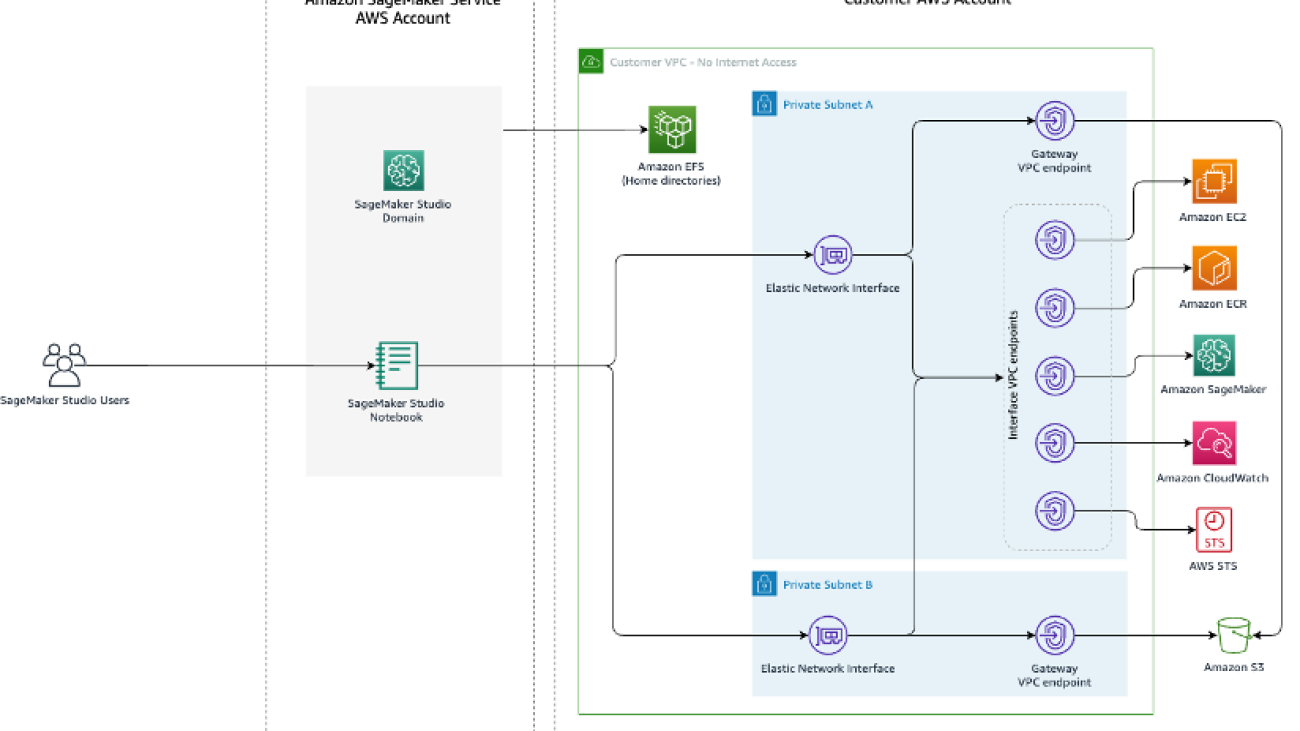
Use generative AI foundation models in VPC mode with no internet connectivity using Amazon SageMaker JumpStart
With recent advancements in generative AI, there are lot of discussions happening on how to use generative AI across different industries to solve specific business problems. Generative AI is a type of AI that can create new content and ideas, including conversations, stories, images, videos, and music. It is all backed by very large models that are pre-trained on vast amounts of data and commonly referred to as foundation models (FMs). These FMs can perform a wide range of tasks that span multiple domains, like writing blog posts, generating images, solving math problems, engaging in dialog, and answering questions based on a document. The size and general-purpose nature of FMs make them different from traditional ML models, which typically perform specific tasks, like analyzing text for sentiment, classifying images, and forecasting trends.
While organizations are looking to use the power of these FMs, they also want the FM-based solutions to be running in their own protected environments. Organizations operating in heavily regulated spaces like global financial services and healthcare and life sciences have auditory and compliance requirements to run their environment in their VPCs. In fact, a lot of times, even direct internet access is disabled in these environments to avoid exposure to any unintended traffic, both ingress and egress.
Amazon SageMaker JumpStart is an ML hub offering algorithms, models, and ML solutions. With SageMaker JumpStart, ML practitioners can choose from a growing list of best performing open source FMs. It also provides the ability to deploy these models in your own Virtual Private Cloud (VPC).
In this post, we demonstrate how to use JumpStart to deploy a Flan-T5 XXL model in a VPC with no internet connectivity. We discuss the following topics:
- How to deploy a foundation model using SageMaker JumpStart in a VPC with no internet access
- Advantages of deploying FMs via SageMaker JumpStart models in VPC mode
- Alternate ways to customize deployment of foundation models via JumpStart
Apart from FLAN-T5 XXL, JumpStart provides lot of different foundation models for various tasks. For the complete list, check out Getting started with Amazon SageMaker JumpStart.
Solution overview
As part of the solution, we cover the following steps:
- Set up a VPC with no internet connection.
- Set up Amazon SageMaker Studio using the VPC we created.
- Deploy the generative AI Flan T5-XXL foundation model using JumpStart in the VPC with no internet access.
The following is an architecture diagram of the solution.

Let’s walk through the different steps to implement this solution.
Prerequisites
To follow along with this post, you need the following:
- Access to an AWS account. For details, check out Creating an AWS account.
- An AWS Identity and Access Management (IAM) role with permissions to deploy the AWS CloudFormation templates used in this solution and manage resources as part of the solution.
Set up a VPC with no internet connection
Create a new CloudFormation stack by using the 01_networking.yaml template. This template creates a new VPC and adds two private subnets across two Availability Zones with no internet connectivity. It then deploys gateway VPC endpoints for accessing Amazon Simple Storage Service (Amazon S3) and interface VPC endpoints for SageMaker and a few other services to allow the resources in the VPC to connect to AWS services via AWS PrivateLink.
Provide a stack name, such as No-Internet, and complete the stack creation process.

This solution is not highly available because the CloudFormation template creates interface VPC endpoints only in one subnet to reduce costs when following the steps in this post.
Set up Studio using the VPC
Create another CloudFormation stack using 02_sagemaker_studio.yaml, which creates a Studio domain, Studio user profile, and supporting resources like IAM roles. Choose a name for the stack; for this post, we use the name SageMaker-Studio-VPC-No-Internet. Provide the name of the VPC stack you created earlier (No-Internet) as the CoreNetworkingStackName parameter and leave everything else as default.

Wait until AWS CloudFormation reports that the stack creation is complete. You can confirm the Studio domain is available to use on the SageMaker console.

To verify the Studio domain user has no internet access, launch Studio using the SageMaker console. Choose File, New, and Terminal, then attempt to access an internet resource. As shown in the following screenshot, the terminal will keep waiting for the resource and eventually time out.

This proves that Studio is operating in a VPC that doesn’t have internet access.
Deploy the generative AI foundation model Flan T5-XXL using JumpStart
We can deploy this model via Studio as well as via API. JumpStart provides all the code to deploy the model via a SageMaker notebook accessible from within Studio. For this post, we showcase this capability from the Studio.
- On the Studio welcome page, choose JumpStart under Prebuilt and automated solutions.

- Choose the Flan-T5 XXL model under Foundation Models.

- By default, it opens the Deploy tab. Expand the Deployment Configuration section to change the
hosting instanceandendpoint name, or add any additional tags. There is also an option to change theS3 bucket locationwhere the model artifact will be stored for creating the endpoint. For this post, we leave everything at its default values. Make a note of the endpoint name to use while invoking the endpoint for making predictions.

- Expand the Security Settings section, where you can specify the
IAM rolefor creating the endpoint. You can also specify theVPC configurationsby providing thesubnetsandsecurity groups. The subnet IDs and security group IDs can be found from the VPC stack’s Outputs tab on the AWS CloudFormation console. SageMaker JumpStart requires at least two subnets as part of this configuration. The subnets and security groups control access to and from the model container.

NOTE: Irrespective of whether the SageMaker JumpStart model is deployed in the VPC or not, the model always runs in network isolation mode, which isolates the model container so no inbound or outbound network calls can be made to or from the model container. Because we’re using a VPC, SageMaker downloads the model artifact through our specified VPC. Running the model container in network isolation doesn’t prevent your SageMaker endpoint from responding to inference requests. A server process runs alongside the model container and forwards it the inference requests, but the model container doesn’t have network access.
- Choose Deploy to deploy the model. We can see the near-real-time status of the endpoint creation in progress. The endpoint creation may take 5–10 minutes to complete.

Observe the value of the field Model data location on this page. All the SageMaker JumpStart models are hosted on a SageMaker managed S3 bucket (s3://jumpstart-cache-prod-{region}). Therefore, irrespective of which model is picked from JumpStart, the model gets deployed from the publicly accessible SageMaker JumpStart S3 bucket and the traffic never goes to the public model zoo APIs to download the model. This is why the model endpoint creation started successfully even when we’re creating the endpoint in a VPC that doesn’t have direct internet access.
The model artifact can also be copied to any private model zoo or your own S3 bucket to control and secure model source location further. You can use the following command to download the model locally using the AWS Command Line Interface (AWS CLI):
aws s3 cp s3://jumpstart-cache-prod-eu-west-1/huggingface-infer/prepack/v1.0.2/infer-prepack-huggingface-text2text-flan-t5-xxl.tar.gz .- After a few minutes, the endpoint gets created successfully and shows the status as In Service. Choose
Open Notebookin theUse Endpoint from Studiosection. This is a sample notebook provided as part of the JumpStart experience to quickly test the endpoint.

- In the notebook, choose the image as Data Science 3.0 and the kernel as Python 3. When the kernel is ready, you can run the notebook cells to make predictions on the endpoint. Note that the notebook uses the invoke_endpoint() API from the AWS SDK for Python to make predictions. Alternatively, you can use the SageMaker Python SDK’s predict() method to achieve the same result.

This concludes the steps to deploy the Flan-T5 XXL model using JumpStart within a VPC with no internet access.
Advantages of deploying SageMaker JumpStart models in VPC mode
The following are some of the advantages of deploying SageMaker JumpStart models in VPC mode:
- Because SageMaker JumpStart doesn’t download the models from a public model zoo, it can be used in fully locked-down environments as well where there is no internet access
- Because the network access can be limited and scoped down for SageMaker JumpStart models, this helps teams improve the security posture of the environment
- Due to the VPC boundaries, access to the endpoint can also be limited via subnets and security groups, which adds an extra layer of security
Alternate ways to customize deployment of foundation models via SageMaker JumpStart
In this section, we share some alternate ways to deploy the model.
Use SageMaker JumpStart APIs from your preferred IDE
Models provided by SageMaker JumpStart don’t require you to access Studio. You can deploy them to SageMaker endpoints from any IDE, thanks to the JumpStart APIs. You could skip the Studio setup step discussed earlier in this post and use the JumpStart APIs to deploy the model. These APIs provide arguments where VPC configurations can be supplied as well. The APIs are part of the SageMaker Python SDK itself. For more information, refer to Pre-trained models.
Use notebooks provided by SageMaker JumpStart from SageMaker Studio
SageMaker JumpStart also provides notebooks to deploy the model directly. On the model detail page, choose Open notebook to open a sample notebook containing the code to deploy the endpoint. The notebook uses SageMaker JumpStart Industry APIs that allow you to list and filter the models, retrieve the artifacts, and deploy and query the endpoints. You can also edit the notebook code per your use case-specific requirements.

Clean up resources
Check out the CLEANUP.md file to find detailed steps to delete the Studio, VPC, and other resources created as part of this post.
Troubleshooting
If you encounter any issues in creating the CloudFormation stacks, refer to Troubleshooting CloudFormation.
Conclusion
Generative AI powered by large language models is changing how people acquire and apply insights from information. However, organizations operating in heavily regulated spaces are required to use the generative AI capabilities in a way that allows them to innovate faster but also simplifies the access patterns to such capabilities.
We encourage you to try out the approach provided in this post to embed generative AI capabilities in your existing environment while still keeping it inside your own VPC with no internet access. For further reading on SageMaker JumpStart foundation models, check out the following:
- Domain-adaptation Fine-tuning of Foundation Models in Amazon SageMaker JumpStart on Financial data
- Implementing MLOps practices with Amazon SageMaker JumpStart pre-trained models
About the authors
 Vikesh Pandey is a Machine Learning Specialist Solutions Architect at AWS, helping customers from financial industries design and build solutions on generative AI and ML. Outside of work, Vikesh enjoys trying out different cuisines and playing outdoor sports.
 Mehran Nikoo is a Senior Solutions Architect at AWS, working with Digital Native businesses in the UK and helping them achieve their goals. Passionate about applying his software engineering experience to machine learning, he specializes in end-to-end machine learning and MLOps practices.

What’s new in TensorFlow 2.13 and Keras 2.13?
 Posted by the TensorFlow and Keras Teams

TensorFlow 2.13 and Keras 2.13 have been released! Highlights of this release include publishing Apple Silicon wheels, the new Keras V3 format being default for .keras extension files and many more!
TensorFlow Core
Apple Silicon wheels for TensorFlow
TensorFlow 2.13 is the first version to provide Apple Silicon wheels, which means when you install TensorFlow on an Apple Silicon Mac, you will be able to use the latest version of TensorFlow. The nightly builds for Apple Silicon wheels were released in March 2023 and this new support will enable more fine-grained testing, thanks to technical collaboration between Apple, MacStadium, and Google.
tf.lite
The Python TensorFlow Lite Interpreter bindings now have an option to use experimental_disable_delegate_clustering flag to turn-off delegate clustering during delegate graph partitioning phase. You can set this flag in TensorFlow Lite interpreter Python API
interpreter = new Interpreter(file_of_a_tensorflowlite_model, experimental_preserve_all_tensors=False) |
The flag is set to False by default. This is an advanced feature in experimental that is designed for people who insert explicit control dependencies via with tf.control_dependencies() or need to change graph execution order.
Besides, there are several operator improvements in TensorFlow Lite in 2.13
- add operation now supports broadcasting up to 6 dimensions. This will remove explicit broadcast ops from many models. The new implementation is also much faster than the current one which calculates the entire index for both inputs the the input instead of only calculating the part that changes.
- Improve the coverage for 16×8 quantization by enabling int16x8 ops for exp, mirror_pad, space_to_batch_nd, batch_to_space_nd
- Increase the coverage of integer data types
- enabled int16 for less, greater_than, equal, bitcast, bitwise_xor, right_shift, top_k, mul, and int16 indices for gather and gather_nd
- enabled int8 for floor_div and floor_mod, bitwise_xor, bitwise_xor
- enabled 32-bit int for bitcast, bitwise_xor, right_shift
tf.data
We have improved usability and added functionality for tf.data APIs.
tf.data.Dataset.zip now supports Python-style zipping. Previously users were required to provide an extra set of parentheses when zipping datasets as in Dataset.zip((a, b, c)). With this change, users can specify the datasets to be zipped simply as Dataset.zip(a, b, c) making it more intuitive.
Additionally, tf.data.Dataset.shuffle now supports full shuffling. To specify that data should be fully shuffled, use dataset = dataset.shuffle(dataset.cardinality()). This will load the full dataset into memory so that it can be shuffled, so make sure to only use this with datasets of filenames or other small datasets.
We have also added a new tf.data.experimental.pad_to_cardinality transformation which pads a dataset with zero elements up to a specified cardinality. This is useful for avoiding partial batches while not dropping any data.
Example usage:
ds = tf.data.Dataset.from_tensor_slices({‘a’: [1, 2]})
ds = ds.apply(tf.data.experimental.pad_to_cardinality(3))
list(ds.as_numpy_iterator())
[{‘a’: 1, ‘valid’: True}, {‘a’: 2, ‘valid’: True}, {‘a’: 0, ‘valid’: False}]This can be useful, e.g. during eval, when partial batches are undesirable but it is also important not to drop any data.
oneDNN BF16 Math Mode on CPU
oneDNN supports BF16 math mode where full FP32 tensors are implicitly down-converted to BF16 during computations for faster execution time. TensorFlow CPU users can enable this by setting the environment variable TF_SET_ONEDNN_FPMATH_MODE to BF16. This mode may negatively impact model accuracy. To go back to full FP32 math mode, unset the variable.
Keras
Keras Saving format
The new Keras V3 saving format, released in TF 2.12, is now the default for all files with the .keras extension.
You can start using it now by calling model.save(“your_model.keras”).
It provides richer Python-side model saving and reloading with numerous advantages:
- A lightweight, faster format:
 |
- Human-readable: The new format is name-based, with a more detailed serialization format that makes debugging much easier. What you load is exactly what you saved, from Python’s perspective.
- Safer: Unlike SavedModel, there is no reliance on loading via bytecode or pickling – a big advancement for secure ML, as pickle files can be exploited to cause arbitrary code execution at loading time.
- More general: Support for non-numerical states, such as vocabularies and lookup tables, is included in the new format.
- Extensible: You can add support for saving and loading exotic state elements in custom layers using save_assets(), such as a FIFOQueue – or anything else you want. You have full control of disk I/O for custom assets.
The legacy formats (h5 and Keras SavedModel) will stay supported in perpetuity. However, we recommend that you consider adopting the new Keras v3 format for saving/reloading in Python runtimes, and using model.export() for inference in all other runtimes (such as TF Serving).

NVIDIA DGX Cloud Now Available to Supercharge Generative AI Training
NVIDIA DGX Cloud — which delivers tools that can turn nearly any company into an AI company — is now broadly available, with thousands of NVIDIA GPUs online on Oracle Cloud Infrastructure, as well as NVIDIA infrastructure located in the U.S. and U.K.
Unveiled at NVIDIA’s GTC conference in March, DGX Cloud is an AI supercomputing service that gives enterprises immediate access to the infrastructure and software needed to train advanced models for generative AI and other groundbreaking applications.
“Generative AI has made the rapid adoption of AI a business imperative for leading companies in every industry, driving many enterprises to seek more accelerated computing infrastructure,” said Pat Moorhead, chief analyst at Moor Insights & Strategy.
Generative AI could add more than $4 trillion to the economy annually, turning proprietary business knowledge across a vast swath of the world’s industries into next-generation AI applications, according to recent estimates by global management consultancy McKinsey.
Industry Pioneers Transforming Business With Generative AI
Nearly every industry can benefit from generative AI, with early pioneers already leading transformative change across their markets.
Healthcare companies use DGX Cloud to train protein models to speed drug discovery and clinical reporting with natural language processing.
Financial service providers use DGX Cloud to forecast trends, optimize portfolios, build recommender systems and develop intelligent generative AI chatbots.
Insurance companies are building models to automate claims processing.
Software companies are using it to develop AI-powered features and applications.
And others are using DGX Cloud to build AI factories and digital twins of valuable assets.
Dedicated AI Supercomputing With Immediate Availability
DGX Cloud instances provide dedicated infrastructure enterprises rent on a monthly basis, ensuring customers can quickly and easily develop large, multi-node training workloads without having to wait for accelerated computing resources that are often in high demand.
“The availability of NVIDIA DGX Cloud provides a new pool of AI supercomputing resources, with nearly instantaneous access,” Moorhead said.
This simple approach to AI supercomputing removes the complexity of acquiring, deploying and managing on-premises infrastructure. Providing NVIDIA DGX AI supercomputing paired with NVIDIA AI Enterprise software, DGX Cloud makes it possible for businesses everywhere to access their own AI supercomputer using a web browser.
NVIDIA AI Supercomputing and Software in a Browser
Each instance of DGX Cloud features eight NVIDIA 80GB Tensor Core GPUs for 640GB of GPU memory per node. A high-performance, low-latency fabric ensures workloads can scale across clusters of interconnected systems, allowing multiple instances to act as one massive GPU. High-performance storage is integrated into DGX Cloud to provide a complete solution.
Enterprises manage and monitor DGX Cloud training workloads using NVIDIA Base Command Platform software. The platform provides a seamless user experience across DGX Cloud and on-premises NVIDIA DGX supercomputers, so enterprises can combine resources when needed.
And DGX Cloud includes NVIDIA AI Enterprise, the software layer of the NVIDIA AI platform, which provides over 100 end-to-end AI frameworks and pretrained models to accelerate data science pipelines and streamline the development and deployment of production AI.
Learn more about how to get started with DGX Cloud.

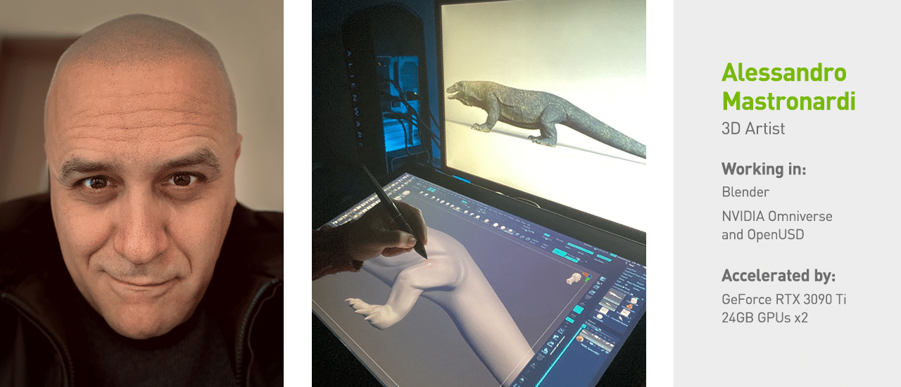
Fin-tastic: 3D Artist Dives Into AI-Powered Oceanic Work This Week ‘In the NVIDIA Studio’
Editor’s note: This post is part of our weekly In the NVIDIA Studio series, which celebrates featured artists, offers creative tips and tricks, and demonstrates how NVIDIA Studio technology improves creative workflows. We’re also deep diving on new GeForce RTX 40 Series GPU features, technologies and resources, and how they dramatically accelerate content creation.
We’re gonna need a bigger boat this week In the NVIDIA Studio as Alessandro Mastronardi, senior artist and programmer at BBC Studios, shares heart-stopping shark videos and renders.
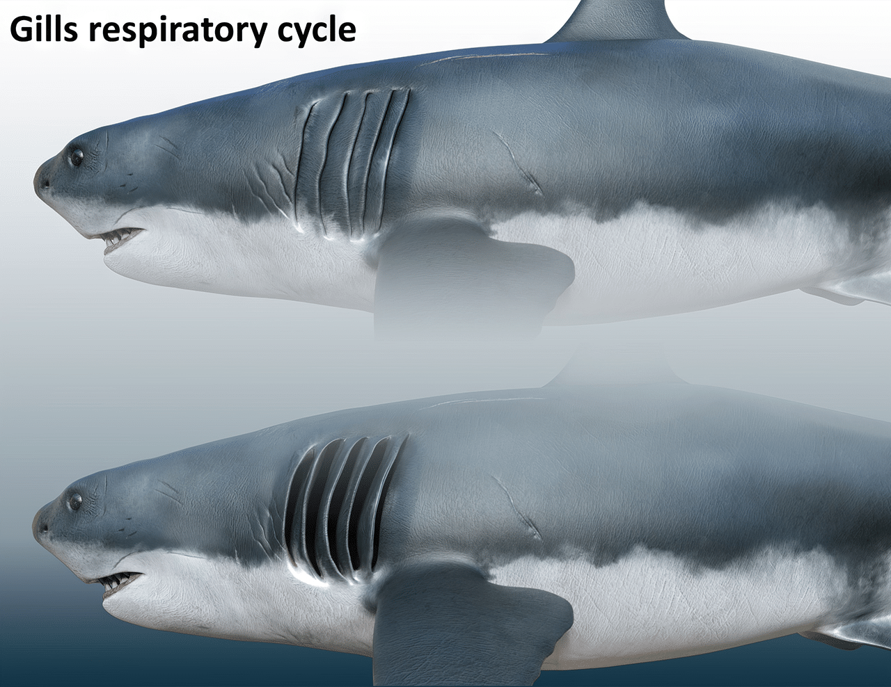
The shark-themed series was conceived during the artist’s recent impromptu trip to Iceland, where he saw a huge basking shark up close. “I was eager to know all about its anatomy, the way it moves and feeds,” said Mastronardi.
After deep-diving on the sharks — including great whites, hammerheads and the Elasmobranchii subclass of rays and the like — he was ready to create. Learn more about his creative journey below — there’s no-fin to lose.
His incredible visuals — alongside extraordinary shark-themed artwork from creators Maggie Molloy and Hypertaf — are featured below in the latest Studio Standout video, which spotlights incredible artists and their work.
Plus, the NVIDIA Studio #StartToFinish community challenge runs through the end of August. Use the hashtag to submit a screenshot of a favorite project featuring its beginning and ending stages for a chance to be featured on the @NVIDIAStudio and @NVIDIAOmniverse social channels.
Jaw-some Creativity
Mastronardi, based in Florence, Italy, works to bring the awe-inspiring beauty of mother nature to the masses.
“The satisfaction of studying nature in all its forms — then transforming that information and reference material into art and content used in several productions and scopes — has been my greatest pride and joy,” he said.

He starts the process by sketching ideas and concepts on paper. “This is something I’ve done since my first years, as it helps to have a clear vision of what I want to achieve,” said Mastronardi.

“Simply put, GeForce RTX GPUs are the most reliable, highest-performing, advanced graphics cards that any 3D professional can use.” — Alessandro Mastronardi
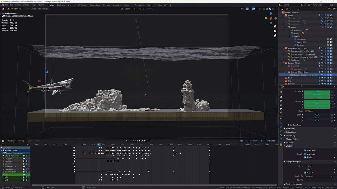
Next, Mastronardi uses ZBrush to model all of his characters. “I like to define a base shape, carefully tune proportions and anatomy, and add detail and resolution until I have a high-polygon, fully detailed, featured character that’s finely sculpted and textured,” he said. “This stage isn’t complete until I’m fully satisfied with how the character looks from every angle, and it has its own personality, so to speak.”
The artist exports characters to Blender to retopologize the high-polygon mesh into low-poly, highly optimized characters. “The key is to reproject the highest possible level of detail onto the character, so that all the details will be maintained.”

Next, Mastronardi rigs the character and sets up a skeleton, configuring all digital bones and inverse kinematics, which determine the motion of objects in the scene.
“The render stage is GPU accelerated and uses OptiX ray-tracing application programming interfaces, which allow fantastic quality and performance.” — Alessandro Mastronardi
Here, Mastronardi’s PC — equipped with two GeForce RTX 3090 Ti 24GB GPUs — does the heavy lifting. Blender Cycles RTX-accelerated AI-powered OptiX ray tracing in the viewport ensures interactive, photorealistic rendering for modeling and animation.
This rigorous process delivers lifelike animations. “A lot of care has to go into the control-rig stage,” said Mastronardi. “All controls must allow for plausible and realistic deformations, with proper anatomy limits and characteristics, so that the character’s movement will look and feel realistic.”
Also using Blender, the artist sets up shaders and materials, and conducts test renders to evaluate how the characters look in different poses. When satisfied, Mastronardi prepares promotional images — built in an environment that matches the characters — and assembles a scene with added effects and props.

Often, Mastronardi inspects his models with NVIDIA Omniverse, a platform for connecting and building custom 3D tools and applications with Universal Scene Description (OpenUSD). “Omniverse is my preferred platform to inspect scenes very quickly,” he said. “I like how agile and effective the interface is, as well as the quality it can deliver.”

Mastronardi exports final files using RTX-accelerated OptiX ray tracing in Blender Cycles for the fastest final frame render. “I love the Cycles render engine, all its features, and the quality and speed that it’s able to deliver,” he added.
Mastronardi plans to use the NVIDIA Broadcast app — from the NVIDIA Studio suite of AI-powered tools — for a new series of 3D art lectures on wildlife, coming soon. Check out Mastronardi’s animal-themed portfolio on ArtStation.
To other artists, Mastronardi would say, “Discard and forget about naysayers, those who tell you ‘No, it can’t be done.’” He added that “growing up, this was a lesson I taught myself: to believe in my own skills, and not to let negativity affect my work or vision to become a wildlife 3D artist.”
There’s some-fin special about those words.
Follow NVIDIA Studio on Instagram, Twitter and Facebook. Access tutorials on the Studio YouTube channel and get updates directly in your inbox by subscribing to the Studio newsletter.
Learn about the latest with OpenUSD and Omniverse at SIGGRAPH, running August 6-10. Take advantage of showfloor experiences like hands-on labs, special events and demo booths — and don’t miss NVIDIA founder and CEO Jensen Huang’s keynote address on Tuesday, Aug. 8, at 8 a.m. PT.
Announcing CPP-based S3 IO DataPipes
Training large deep learning models requires large datasets. Amazon Simple Storage Service (Amazon S3) is a scalable cloud object store service used for storing large training datasets. Machine learning (ML) practitioners need an efficient data pipe that can download data from Amazon S3, transform the data, and feed the data to GPUs for training models with high throughput and low latency.
In this post, we introduce the new S3 IO DataPipes for PyTorch, S3FileLister and S3FileLoader. For memory efficiency and fast runs, the new DataPipes use the C++ extension to access Amazon S3. Benchmarking shows that S3FileLoader is 59.8% faster than FSSpecFileOpener for downloading a natural language processing (NLP) dataset from Amazon S3. You can build IterDataPipe training pipelines with the new DataPipes. We also demonstrate that the new DataPipe can reduce overall Bert and ResNet50 training time by 7%. The new DataPipes have been upstreamed to the open-source TorchData 0.4.0 with PyTorch 1.12.0.
Overview
Amazon S3 is a scalable cloud storage service with no limit on data volume. Loading data from Amazon S3 and feeding the data to high-performance GPUs such as NVIDIA A100 can be challenging. It requires an efficient data pipeline that can meet the data processing speed of GPUs. To help with this, we released a new high performance tool for PyTorch: S3 IO DataPipes. DataPipes are subclassed from torchdata.datapipes.iter.IterDataPipe, so they can interact with the IterableDataPipe interface. Developers can quickly build their DataPipe DAGs to access, transform, and manipulate data with shuffle, sharding, and batch features.
The new DataPipes are designed to be file format agnostic and Amazon S3 data is downloaded as binary large objects (BLOBs). It can be used as a composable building block to assemble a DataPipe graph that can load tabular, NLP, and computer vision (CV) data into your training pipelines.
Under the hood, the new S3 IO DataPipes employ a C++ S3 handler with the AWS C++ SDK. In general, a C++ implementation is more memory efficient and has better CPU core usage (no Global Interpreter Lock) in threading compared to Python. The new C++ S3 IO DataPipes are recommended for high throughput, low latency data loading in training large deep learning models.
The new S3 IO DataPipes provide two first-class citizen APIs:
- S3FileLister – Iterable that lists S3 file URLs within the given S3 prefixes. The functional name for this API is
list_files_by_s3. - S3FileLoader – Iterable that loads S3 files from the given S3 prefixes. The functional name for this API is
load_files_by_s3.
Usage
In this section, we provide instructions for using the new S3 IO DataPipes. We also provide a code snippet for load_files_by_s3().
Build from source
The new S3 IO DataPipes use the C++ extension. It is built into the torchdata package by default. However, if the new DataPipes are not available within the environment, for example Windows on Conda, you need to build from the source. For more information, refer to Iterable Datapipes.
Configuration
Amazon S3 supports global buckets. However, a bucket is created within a Region. You can pass a Region to the DataPipes by using __init__(). Alternatively, you can either export AWS_REGION=us-west-2 into your shell or set an environment variable with os.environ['AWS_REGION'] = 'us-east-1' in your code.
To read objects in a bucket that aren’t publicly accessible, you must provide AWS credentials through one of the following methods:
- Install and configure the AWS Command Line Interface (AWS CLI) with
AWS configure - Set credentials in the AWS credentials profile file on the local system, located at
~/.aws/credentialson Linux, macOS, or Unix - Set the
AWS_ACCESS_KEY_IDandAWS_SECRET_ACCESS_KEYenvironment variables - If you’re using this library on an Amazon Elastic Compute Cloud (Amazon EC2) instance, specify an AWS Identity and Access Management (IAM) role and then give the EC2 instance access to that role
Example code
The following code snippet provides a typical usage of load_files_by_s3():
from torch.utils.data import DataLoader

from torchdata.datapipes.iter import IterableWrapper


s3_shard_urls = IterableWrapper(["s3://bucket/prefix/",])

s3_shards = s3_shard_urls.load_files_by_s3()

# text data

training_data = s3_shards.readlines(return_path=False)

data_loader = DataLoader(
      training_data,
      batch_size=batch_size,
      num_workers=num_workers,

)
# training loop

for epoch in range(epochs):

      # training step

      for bach_data in data_loader:

         # forward pass, backward pass, model update
Benchmark
In this section, we demonstrate how the new DataPipe can reduce overall Bert and ResNet50 training time.
Isolated DataLoader performance evaluation against FSSpec
FSSpecFileOpener is another PyTorch S3 DataPipe. It uses botocore and aiohttp/asyncio to access S3 data. The following is the performance test setup and result (quoted from Performance Comparison between native AWSSDK and FSSpec (boto3) based DataPipes).
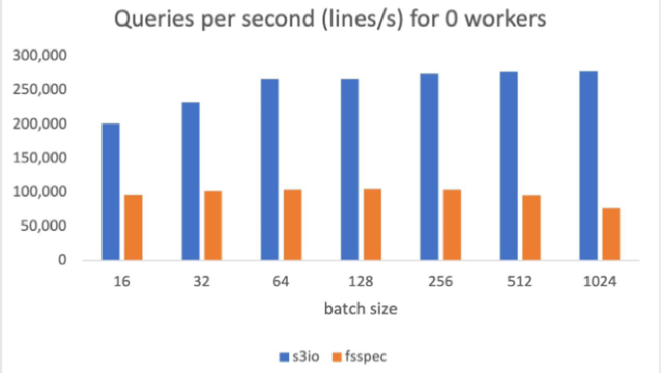
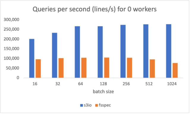
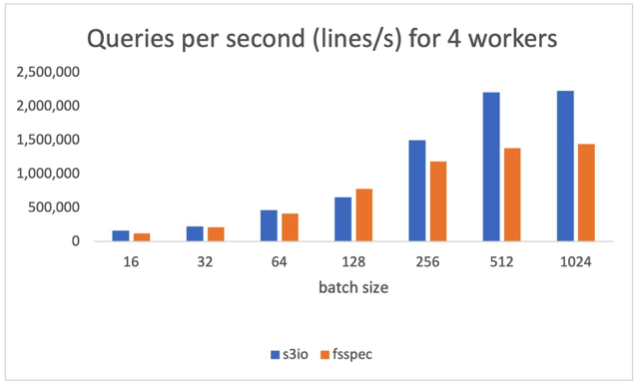
The S3 data in the test is a sharded text dataset. Each shard has about 100,000 lines and each line is around 1.6 KB, making each shard about 156 MB. The measurements in this benchmark are averaged over 1,000 batches. No shuffling, sampling, or transforms were performed.
The following chart reports the throughput comparison for various batch sizes for num_workers=0, the data loader runs in the main process. S3FileLoader has higher queries per second (QPS). It is 90% higher than fsspec at batch size 512.
The following chart reports the results for num_workers=4, the data loaders runs in the main process. S3FileLoader is 59.8% higher than fsspec at batch size 512.
Training ResNet50 Model against Boto3
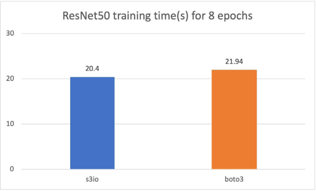
For the following chart, we trained a ResNet50 model on a cluster of 4 p3.16xlarge instances with a total 32 GPUs. The training dataset is ImageNet with 1.2 million images organized into 1,000-image shards. The training batch size is 64. The training time is measured in seconds. For eight epochs, S3FileLoader is 7.5% faster than Boto3.
Training a Bert model against Boto3
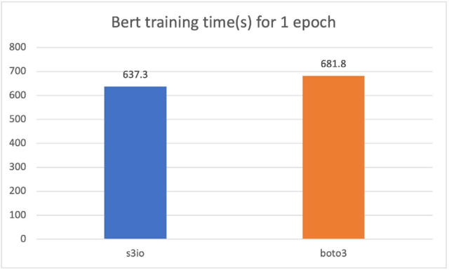
For the following cart, we trained a Bert model on a cluster of 4 p3.16xlarge instances with a total 32 GPUs. The training corpus has 1474 files. Each file has around 150,000 samples. To run a shorter epoch, we use 0.05% (approximately 75 samples) per file. The batch size is 2,048. The training time is measured in seconds. For one epoch, S3FileLoader is 7% faster than Boto3.
Comparison against the original PyTorch S3 plugin
The new PyTorch S3 DataPipes perform substantially better than the original PyTorch S3 plugin. We have tuned the internal buffer size for S3FileLoader. The loading time is measured in seconds.
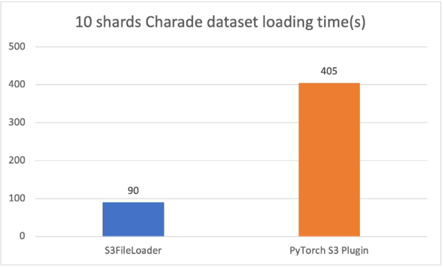
For the 10 sharded charades files (approximately 1.5 GiB each), S3FileLoader was 3.5 times faster in our experiments.
Best practices
Training large deep learning models may require a massive compute cluster with tens or even hundreds of nodes. Each node in the cluster may generate a large number of data loading requests that hit a specific S3 shard. To avoid throttle, we recommend sharding training data across S3 buckets and S3 folders.
To achieve good performance, it helps to have file sizes that are big enough to parallelize across a given file, but not so big that we hit the limits of throughput on that object on Amazon S3 depending on the training job. The optimal size can be between 50–200 MB.
Conclusion and next steps
In this post, we introduced you to the new PyTorch IO DataPipes. The new DataPipes use aws-sdk-cpp and show better performance against Boto3-based data loaders.
For next steps, we plan to improve on usability, performance, and functionality by focusing on the following features:
- S3 authorization with IAM roles – Currently, the S3 DataPipes support explicit access credentials, instance profiles, and S3 bucket policies. However, there are use cases where IAM roles are preferred.
- Double buffering – We plan to offer double buffering to support multi-worker downloading.
- Local caching – We plan on making model training able to traverse the training dataset for multiple passes. Local caching after the first epoch can cut out time of flight delays from Amazon S3, which can substantially accelerate data retrieval time for subsequent epochs.
- Customizable configuration – We plan to expose more parameters such as internal buffer size, multi-part chunk size, and executor count and allow users to further tune data loading efficiency.
- Amazon S3 upload – We plan to expand the S3 DataPipes to support upload for checkpointing.
- Merge with fsspec –
fsspecis used in other systems such astorch.save(). We can integrate the new S3 DataPipes withfsspecso they can have more use cases.
Acknowledgement
We would like to thank Vijay Rajakumar and Kiuk Chung from Amazon for providing their guidance for S3 Common RunTime and PyTorch DataLoader. We also want to thank Erjia Guan, Kevin Tse, Vitaly Fedyunin , Mark Saroufim, Hamid Shojanazeri, Matthias Reso, and Geeta Chauhan from Meta AI/ML, and Joe Evans from AWS for reviewing the blog and the GitHub PRs.
References

How Patsnap used GPT-2 inference on Amazon SageMaker with low latency and cost
This blog post was co-authored, and includes an introduction, by Zilong Bai, senior natural language processing engineer at Patsnap.
You’re likely familiar with the autocomplete suggestion feature when you search for something on Google or Amazon. Although the search terms in these scenarios are pretty common keywords or expressions that we use in daily life, in some cases search terms are very specific to the scenario. Patent search is one of them. Recently, the AWS Generative AI Innovation Center collaborated with Patsnap to implement a feature to automatically suggest search keywords as an innovation exploration to improve user experiences on their platform.
Patsnap provides a global one-stop platform for patent search, analysis, and management. They use big data (such as a history of past search queries) to provide many powerful yet easy-to-use patent tools. These tools have enabled Patsnap’s global customers to have a better understanding of patents, track recent technological advances, identify innovation trends, and analyze competitors in real time.
At the same time, Patsnap is embracing the power of machine learning (ML) to develop features that can continuously improve user experiences on the platform. A recent initiative is to simplify the difficulty of constructing search expressions by autofilling patent search queries using state-of-the-art text generation models. Patsnap had trained a customized GPT-2 model for such a purpose. Because there is no such existing feature in a patent search engine (to their best knowledge), Patsnap believes adding this feature will increase end-user stickiness.
However, in their recent experiments, the inference latency and queries per second (QPS) of a PyTorch-based GPT-2 model couldn’t meet certain thresholds that can justify its business value. To tackle this challenge, AWS Generative AI Innovation Center scientists explored a variety of solutions to optimize GPT-2 inference performance, resulting in lowering the model latency by 50% on average and improving the QPS by 200%.
Large language model inference challenges and optimization approaches
In general, applying such a large model in a real-world production environment is non-trivial. The prohibitive computation cost and latency of PyTorch-based GPT-2 made it difficult to be widely adopted from a business operation perspective. In this project, our objective is to significantly improve the latency with reasonable computation costs. Specifically, Patsnap requires the following:
- The average latency of model inference for generating search expressions needs to be controlled within 600 milliseconds in real-time search scenarios
- The model requires high throughput and QPS to do a large number of searches per second during peak business hours
In this post, we discuss our findings using Amazon Elastic Compute Cloud (Amazon EC2) instances, featuring GPU-based instances using NVIDIA TensorRT.
In a short summary, we use NVIDIA TensorRT to optimize the latency of GPT-2 and deploy it to an Amazon SageMaker endpoint for model serving, which reduces the average latency from 1,172 milliseconds to 531 milliseconds
In the following sections, we go over the technical details of the proposed solutions with key code snippets and show comparisons with the customer’s status quo based on key metrics.
GPT-2 model overview
Open AI’s GPT-2 is a large transformer-based language model with 1.5 billion parameters, trained on the WebText dataset, containing 8 million web pages. The GPT-2 is trained with a simple objective: predict the next word, given all of the previous words within some text. The diversity of the dataset causes this simple goal to contain naturally occurring demonstrations of many tasks across diverse domains. GPT-2 displays a broad set of capabilities, including the ability to generate conditional synthetic text samples of unprecedented quality, where we prime the model with an input and let it generate a lengthy continuation. In this situation, we exploit it to generate search queries. As GPT models keep growing larger, inference costs are continuously rising, which increases the need to deploy these models with acceptable cost.
Achieve low latency on GPU instances via TensorRT
TensorRT is a C++ library for high-performance inference on NVIDIA GPUs and deep learning accelerators, supporting major deep learning frameworks such as PyTorch and TensorFlow. Previous studies have shown great performance improvement in terms of model latency. Therefore, it’s an ideal choice for us to reduce the latency of the target model on NVIDIA GPUs.
We are able to achieve a significant reduction in GPT-2 model inference latency with a TensorRT-based model on NVIDIA GPUs. The TensorRT-based model is deployed via SageMaker for performance tests. In this post, we show the steps to convert the original PyTorch-based GPT-2 model to a TensorRT-based model.
Converting the PyTorch-based GPT-2 to the TensorRT-based model is not difficult via the official tool provided by NVIDIA. In addition, with such straightforward conversions, no obvious model accuracy degradation has been observed. In general, there are three steps to follow:
- Analyze your GPT-2. As of this writing, NVIDIA’s conversion tool only supports Hugging Face’s version of GPT-2 model. If the current GPT-2 model isn’t the original version, you need to modify it accordingly. It’s recommended to strip out custom code from the original GPT-2 implementation of Hugging Face, which is very helpful for the conversion.
- Install the required Python packages. The conversion process first converts the PyTorch-based model to the ONNX model and then converts the ONNX-based model to the TensorRT-based model. The following Python packages are needed for this two-step conversion:
- Convert your model. The following code contains the functions for the two-step conversion:
Latency comparison: PyTorch vs. TensorRT
JMeter is used for performance benchmarking in this project. JMeter is an Apache project that can be used as a load testing tool for analyzing and measuring the performance of a variety of services. We record the QPS and latency of the original PyTorch-based model and our converted TensorRT-based GPT-2 model on an AWS P3.2xlarge instance. As we show later in this post, due to the powerful acceleration ability of TensorRT, the latency of GPT-2 is significantly reduced. When the request concurrency is 1, the average latency has been reduced by 274 milliseconds (2.9 times faster). From the perspective of QPS, it is increased to 7 from 2.4, which is around a 2.9 times boost compared to the original PyTorch-based model. Moreover, as the concurrency increases, QPS keeps increasing. This suggests lower costs with acceptable latency increase (but still much faster than the original model).
The following table compares latency:
| . | Concurrency | QPS | Maximum Latency | Minumum Latency | Average Latency |
| Customer PyTorch version (on p3.2xlarge) | 1 | 2.4 | 632 | 105 | 417 |
| 2 | 3.1 | 919 | 168 | 636 | |
| 3 | 3.4 | 1911 | 222 | 890 | |
| 4 | 3.4 | 2458 | 277 | 1172 | |
| AWS TensorRT version (on p3.2xlarge) | 1 | 7 (+4.6) | 275 | 22 | 143 (-274 ms) |
| 2 | 7.2 (+4.1) | 274 | 51 | 361 (-275 ms) | |
| 3 | 7.3 (+3.9) | 548 | 49 | 404 (-486 ms) | |
| 4 | 7.5 (+4.1) | 765 | 62 | 531 (-641 ms) |
Deploy TensorRT-based GPT-2 with SageMaker and a custom container
TensorRT-based GPT-2 requires a relatively recent TensorRT version, so we choose the bring your own container (BYOC) mode of SageMaker to deploy our model. BYOC mode provides a flexible way to deploy the model, and you can build customized environments in your own Docker container. In this section, we show how to build your own container, deploy your own GPT-2 model, and test with the SageMaker endpoint API.
Build your own container
The container’s file directory is presented in the following code. Specifically, Dockerfile and build.sh are used to build the Docker container. gpt2 and predictor.py implement the model and the inference API. serve, nginx.conf, and wsgi.py provide the configuration for the NGINX web server.
You can run sh ./build.sh to build the container.
Deploy to a SageMaker endpoint
After you have built a container to run the TensorRT-based GPT-2, you can enable real-time inference via a SageMaker endpoint. Use the following code snippets to create the endpoint and deploy the model to the endpoint using the corresponding SageMaker APIs:
Test the deployed model
After the model is successfully deployed, you can test the endpoint via the SageMaker notebook instance with the following code:
Conclusion
In this post, we described how to enable low-latency GPT-2 inference on SageMaker to create business value. Specifically, with the support of NVIDIA TensorRT, we can achieve 2.9 times acceleration on the NVIDIA GPU instances with SageMaker for a customized GPT-2 model.
If you want help with accelerating the use of GenAI models in your products and services, please contact the AWS Generative AI Innovation Center. The AWS Generative AI Innovation Center can help you make your ideas a reality faster and more effectively. To get started with the Generative AI Innovation Center, visit here.
About the Authors
 Hao Huang is an applied scientist at the AWS Generative AI Innovation Center. He specializes in Computer Vision (CV) and Visual-Language Model (VLM). Recently, he has developed a strong interest in generative AI technologies and has already collaborated with customers to apply these cutting-edge technologies to their business. He is also a reviewer for AI conferences such as ICCV and AAAI.
 Zilong Bai is a senior natural language processing engineer at Patsnap. He is passionate about research and proof-of-concept work on cutting-edge techniques for generative language models.
 Yuanjun Xiao is a Solution Architect at AWS. He is responsible for AWS architecture consulting and design. He is also passionate about building AI and analytic solutions.
 Xuefei Zhang is an applied scientist at the AWS Generative AI Innovation Center, works in NLP and AGI areas to solve industry problems with customers.
 Guang Yang is a senior applied scientist at the AWS Generative AI Innovation Center where he works with customers across various verticals and applies creative problem solving to generate value for customers with state-of-the-art ML/AI solutions.
Optimize AWS Inferentia utilization with FastAPI and PyTorch models on Amazon EC2 Inf1 & Inf2 instances
When deploying Deep Learning models at scale, it is crucial to effectively utilize the underlying hardware to maximize performance and cost benefits. For production workloads requiring high throughput and low latency, the selection of the Amazon Elastic Compute Cloud (EC2) instance, model serving stack, and deployment architecture is very important. Inefficient architecture can lead to suboptimal utilization of the accelerators and unnecessarily high production cost.
In this post we walk you through the process of deploying FastAPI model servers on AWS Inferentia devices (found on Amazon EC2 Inf1 and Amazon EC Inf2 instances). We also demonstrate hosting a sample model that is deployed in parallel across all NeuronCores for maximum hardware utilization.
Solution overview
FastAPI is an open-source web framework for serving Python applications that is much faster than traditional frameworks like Flask and Django. It utilizes an Asynchronous Server Gateway Interface (ASGI) instead of the widely used Web Server Gateway Interface (WSGI). ASGI processes incoming requests asynchronously as opposed to WSGI which processes requests sequentially. This makes FastAPI the ideal choice to handle latency sensitive requests. You can use FastAPI to deploy a server that hosts an endpoint on an Inferentia (Inf1/Inf2) instances that listens to client requests through a designated port.
Our objective is to achieve highest performance at lowest cost through maximum utilization of the hardware. This allows us to handle more inference requests with fewer accelerators. Each AWS Inferentia1 device contains four NeuronCores-v1 and each AWS Inferentia2 device contains two NeuronCores-v2. The AWS Neuron SDK allows us to utilize each of the NeuronCores in parallel, which gives us more control in loading and inferring four or more models in parallel without sacrificing throughput.
With FastAPI, you have your choice of Python web server (Gunicorn, Uvicorn, Hypercorn, Daphne). These web servers provide and abstraction layer on top of the underlying Machine Learning (ML) model. The requesting client has the benefit of being oblivious to the hosted model. A client doesn’t need to know the model’s name or version that has been deployed under the server; the endpoint name is now just a proxy to a function that loads and runs the model. In contrast, in a framework-specific serving tool, such as TensorFlow Serving, the model’s name and version are part of the endpoint name. If the model changes on the server side, the client has to know and change its API call to the new endpoint accordingly. Therefore, if you are continuously evolving the version models, such as in the case of A/B testing, then using a generic Python web server with FastAPI is a convenient way of serving models, because the endpoint name is static.
An ASGI server’s role is to spawn a specified number of workers that listen for client requests and run the inference code. An important capability of the server is to make sure the requested number of workers are available and active. In case a worker is killed, the server must launch a new worker. In this context, the server and workers may be identified by their Unix process ID (PID). For this post, we use a Hypercorn server, which is a popular choice for Python web servers.
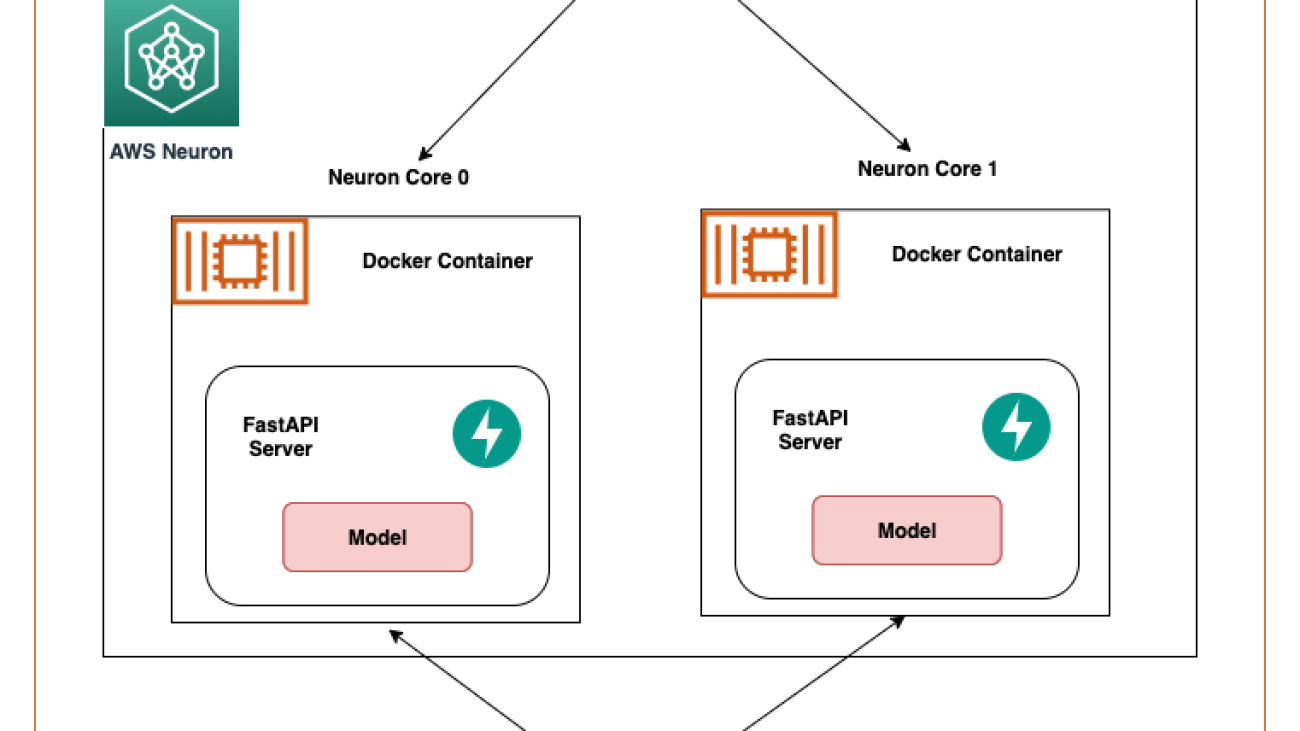
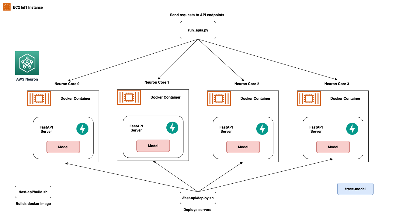
In this post, we share best practices to deploy deep learning models with FastAPI on AWS Inferentia NeuronCores. We show that you can deploy multiple models on separate NeuronCores that can be called concurrently. This setup increases throughput because multiple models can be inferred concurrently and NeuronCore utilization is fully optimized. The code can be found on the GitHub repo. The following figure shows the architecture of how to set up the solution on an EC2 Inf2 instance.
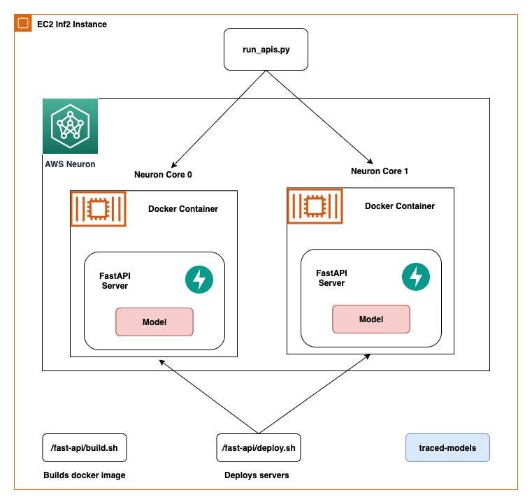
The same architecture applies to an EC2 Inf1 instance type except it has four cores. So that changes the architecture diagram a little bit.
AWS Inferentia NeuronCores
Let’s dig a little deeper into tools provided by AWS Neuron to engage with the NeuronCores. The following tables shows the number of NeuronCores in each Inf1 and Inf2 instance type. The host vCPUs and the system memory are shared across all available NeuronCores.
| Instance Size | # Inferentia Accelerators | # NeuronCores-v1 | vCPUs | Memory (GiB) |
| Inf1.xlarge | 1 | 4 | 4 | 8 |
| Inf1.2xlarge | 1 | 4 | 8 | 16 |
| Inf1.6xlarge | 4 | 16 | 24 | 48 |
| Inf1.24xlarge | 16 | 64 | 96 | 192 |
| Instance Size | # Inferentia Accelerators | # NeuronCores-v2 | vCPUs | Memory (GiB) |
| Inf2.xlarge | 1 | 2 | 4 | 32 |
| Inf2.8xlarge | 1 | 2 | 32 | 32 |
| Inf2.24xlarge | 6 | 12 | 96 | 192 |
| Inf2.48xlarge | 12 | 24 | 192 | 384 |
Inf2 instances contain the new NeuronCores-v2 in comparison to the NeuronCore-v1 in the Inf1 instances. Despite fewer cores, they are able to offer 4x higher throughput and 10x lower latency than Inf1 instances. Inf2 instances are ideal for Deep Learning workloads like Generative AI, Large Language Models (LLM) in OPT/GPT family and vision transformers like Stable Diffusion.
The Neuron Runtime is responsible for running models on Neuron devices. Neuron Runtime determines which NeuronCore will run which model and how to run it. Configuration of Neuron Runtime is controlled through the use of environment variables at the process level. By default, Neuron framework extensions will take care of Neuron Runtime configuration on the user’s behalf; however, explicit configurations are also possible to achieve more optimized behavior.
Two popular environment variables are NEURON_RT_NUM_CORES and NEURON_RT_VISIBLE_CORES. With these environment variables, Python processes can be tied to a NeuronCore. With NEURON_RT_NUM_CORES, a specified number of cores can be reserved for a process, and with NEURON_RT_VISIBLE_CORES, a range of NeuronCores can be reserved. For example, NEURON_RT_NUM_CORES=2 myapp.py will reserve two cores and NEURON_RT_VISIBLE_CORES=’0-2’ myapp.py will reserve zero, one, and two cores for myapp.py. You can reserve NeuronCores across devices (AWS Inferentia chips) as well. So, NEURON_RT_VISIBLE_CORES=’0-5’ myapp.py will reserve the first four cores on device1 and one core on device2 in an Ec2 Inf1 instance type. Similarly, on an EC2 Inf2 instance type, this configuration will reserve two cores across device1 and device2 and one core on device3. The following table summarizes the configuration of these variables.
| Name | Description | Type | Expected Values | Default Value | RT Version |
NEURON_RT_VISIBLE_CORES |
Range of specific NeuronCores needed by the process | Integer range (like 1-3) | Any value or range between 0 to Max NeuronCore in the system | None | 2.0+ |
NEURON_RT_NUM_CORES |
Number of NeuronCores required by the process | Integer | A value from 1 to Max NeuronCore in the system | 0, which is interpreted as “all” | 2.0+ |
For a list of all environment variables, refer to Neuron Runtime Configuration.
By default, when loading models, models get loaded onto NeuronCore 0 and then NeuronCore 1 unless explicitly stated by the preceding environment variables. As specified earlier, the NeuronCores share the available host vCPUs and system memory. Therefore, models deployed on each NeuronCore will compete for the available resources. This won’t be an issue if the model is utilizing the NeuronCores to a large extent. But if a model is running only partly on the NeuronCores and the rest on host vCPUs then considering CPU availability per NeuronCore become important. This affects the choice of the instance as well.
The following table shows number of host vCPUs and system memory available per model if one model was deployed to each NeuronCore. Depending on your application’s NeuronCore usage, vCPU, and memory usage, it is recommended to run tests to find out which configuration is most performant for your application. The Neuron Top tool can help in visualizing core utilization and device and host memory utilization. Based on these metrics an informed decision can be made. We demonstrate the use of Neuron Top at the end of this blog.
| Instance Size | # Inferentia Accelerators | # Models | vCPUs/Model | Memory/Model (GiB) |
| Inf1.xlarge | 1 | 4 | 1 | 2 |
| Inf1.2xlarge | 1 | 4 | 2 | 4 |
| Inf1.6xlarge | 4 | 16 | 1.5 | 3 |
| Inf1.24xlarge | 16 | 64 | 1.5 | 3 |
| Instance Size | # Inferentia Accelerators | # Models | vCPUs/Model | Memory/Model (GiB) |
| Inf2.xlarge | 1 | 2 | 2 | 8 |
| Inf2.8xlarge | 1 | 2 | 16 | 64 |
| Inf2.24xlarge | 6 | 12 | 8 | 32 |
| Inf2.48xlarge | 12 | 24 | 8 | 32 |
To test out the Neuron SDK features yourself, check out the latest Neuron capabilities for PyTorch.
System setup
The following is the system setup used for this solution:
- Instance size – 6xlarge (if using Inf1), Inf2.xlarge (if using Inf2)
- Image for instance – Deep Learning AMI Neuron PyTorch 1.11.0 (Ubuntu 20.04) 20230125
- Model – https://huggingface.co/twmkn9/bert-base-uncased-squad2
- Framework – PyTorch
Set up the solution
There are a couple of things we need to do to setup the solution. Start by creating an IAM role that your EC2 instance is going to assume that will allow it to push and pull from Amazon Elastic Container Registry.
Step 1: Setup the IAM role
- Start by logging into the console and accessing IAM > Roles > Create Role
- Select Trusted entity type
AWS Service - Select EC2 as the service under use-case
- Click Next and you’ll be able to see all policies available
- For the purpose of this solution, we’re going to give our EC2 instance full access to ECR. Filter for AmazonEC2ContainerRegistryFullAccess and select it.
- Press next and name the role
inf-ecr-access
Note: the policy we attached gives the EC2 instance full access to Amazon ECR. We strongly recommend following the principal of least-privilege for production workloads.
Step 2: Setup AWS CLI
If you’re using the prescribed Deep Learning AMI listed above, it comes with AWS CLI installed. If you’re using a different AMI (Amazon Linux 2023, Base Ubuntu etc.), install the CLI tools by following this guide.
Once you have the CLI tools installed, configure the CLI using the command aws configure. If you have access keys, you can add them here but don’t necessarily need them to interact with AWS services. We’re relying on IAM roles to do that.
Note: We need to enter at-least one value (default region or default format) to create the default profile. For this example, we’re going with us-east-2 as the region and json as the default output.
Clone the Github repository
The GitHub repo provides all the scripts necessary to deploy models using FastAPI on NeuronCores on AWS Inferentia instances. This example uses Docker containers to ensure we can create reusable solutions. Included in this example is the following config.properties file for users to provide inputs.
The configuration file needs user-defined name prefixes for the Docker image and Docker containers. The build.sh script in the fastapi and trace-model folders use this to create Docker images.
Compile a model on AWS Inferentia
We will start with tracing the model and producing a PyTorch Torchscript .pt file. Start by accessing trace-model directory and modifying the .env file. Depending upon the type of instance you chose, modify the CHIP_TYPE within the .env file. As an example, we will choose Inf2 as the guide. The same steps apply to the deployment process for Inf1.
Next set the default region in the same file. This region will be used to create an ECR repository and Docker images will be pushed to this repository. Also in this folder, we provide all the scripts necessary to trace a bert-base-uncased model on AWS Inferentia. This script could be used for most models available on Hugging Face. The Dockerfile has all the dependencies to run models with Neuron and runs the trace-model.py code as the entry point.
Neuron compilation explained
The Neuron SDK’s API closely resembles the PyTorch Python API. The torch.jit.trace() from PyTorch takes the model and sample input tensor as arguments. The sample inputs are fed to the model and the operations that are invoked as that input makes its way through the model’s layers are recorded as TorchScript. To learn more about JIT Tracing in PyTorch, refer to the following documentation.
Just like torch.jit.trace(), you can check to see if your model can be compiled on AWS Inferentia with the following code for inf1 instances.
For inf2, the library is called torch_neuronx. Here’s how you can test your model compilation against inf2 instances.
After creating the trace instance, we can pass the example tensor input like so:
And finally save the resulting TorchScript output on local disk
As shown in the preceding code, you can use compiler_args and optimizations to optimize the deployment. For a detailed list of arguments for the torch.neuron.trace API, refer to PyTorch-Neuron trace python API.
Keep the following important points in mind:
- The Neuron SDK doesn’t support dynamic tensor shapes as of this writing. Therefore, a model will have to be compiled separately for different input shapes. For more information on running inference on variable input shapes with bucketing, refer to Running inference on variable input shapes with bucketing.
- If you face out of memory issues when compiling a model, try compiling the model on an AWS Inferentia instance with more vCPUs or memory, or even a large c6i or r6i instance as compilation only uses CPUs. Once compiled, the traced model can probably be run on smaller AWS Inferentia instance sizes.
Build process explanation
Now we will build this container by running build.sh. The build script file simply creates the Docker image by pulling a base Deep Learning Container Image and installing the HuggingFace transformers package. Based on the CHIP_TYPE specified in the .env file, the docker.properties file decides the appropriate BASE_IMAGE. This BASE_IMAGE points to a Deep Learning Container Image for Neuron Runtime provided by AWS.
It is available through a private ECR repository. Before we can pull the image, we need to login and get temporary AWS credentials.
Note: we need to replace the region listed in the command specified by the region flag and within the repository URI with the region we put in the .env file.
For the purpose of making this process easier, we can use the fetch-credentials.sh file. The region will be taken from the .env file automatically.
Next, we’ll push the image using the script push.sh. The push script creates a repository in Amazon ECR for you and pushes the container image.
Finally, when the image is built and pushed, we can run it as a container by running run.sh and tail running logs with logs.sh. In the compiler logs (see the following screenshot), you will see the percentage of arithmetic operators compiled on Neuron and percentage of model sub-graphs successfully compiled on Neuron. The screenshot shows the compiler logs for the bert-base-uncased-squad2 model. The logs show that 95.64% of the arithmetic operators were compiled, and it also gives a list of operators that were compiled on Neuron and those that aren’t supported.
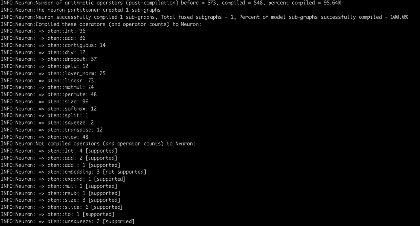
Here is a list of all supported operators in the latest PyTorch Neuron package. Similarly, here is the list of all supported operators in the latest PyTorch Neuronx package.
Deploy models with FastAPI
After the models are compiled, the traced model will be present in the trace-model folder. In this example, we have placed the traced model for a batch size of 1. We consider a batch size of 1 here to account for those use cases where a higher batch size is not feasible or required. For use cases where higher batch sizes are needed, the torch.neuron.DataParallel (for Inf1) or torch.neuronx.DataParallel (for Inf2) API may also be useful.
The fast-api folder provides all the necessary scripts to deploy models with FastAPI. To deploy the models without any changes, simply run the deploy.sh script and it will build a FastAPI container image, run containers on the specified number of cores, and deploy the specified number of models per server in each FastAPI model server. This folder also contains a .env file, modify it to reflect the correct CHIP_TYPE and AWS_DEFAULT_REGION.
Note: FastAPI scripts rely on the same environment variables used to build, push and run the images as containers. FastAPI deployment scripts will use the last known values from these variables. So, if you traced the model for Inf1 instance type last, that model will be deployed through these scripts.
The fastapi-server.py file which is responsible for hosting the server and sending the requests to the model does the following:
- Reads the number of models per server and the location of the compiled model from the properties file
- Sets visible NeuronCores as environment variables to the Docker container and reads the environment variables to specify which NeuronCores to use
- Provides an inference API for the
bert-base-uncased-squad2model - With
jit.load(), loads the number of models per server as specified in the config and stores the models and the required tokenizers in global dictionaries
With this setup, it would be relatively easy to set up APIs that list which models and how many models are stored in each NeuronCore. Similarly, APIs could be written to delete models from specific NeuronCores.
The Dockerfile for building FastAPI containers is built on the Docker image we built for tracing the models. This is why the docker.properties file specifies the ECR path to the Docker image for tracing the models. In our setup, the Docker containers across all NeuronCores are similar, so we can build one image and run multiple containers from one image. To avoid any entry point errors, we specify ENTRYPOINT ["/usr/bin/env"] in the Dockerfile before running the startup.sh script, which looks like hypercorn fastapi-server:app -b 0.0.0.0:8080. This startup script is the same for all containers. If you’re using the same base image as for tracing models, you can build this container by simply running the build.sh script. The push.sh script remains the same as before for tracing models. The modified Docker image and container name are provided by the docker.properties file.
The run.sh file does the following:
- Reads the Docker image and container name from the properties file, which in turn reads the
config.propertiesfile, which has anum_coresuser setting - Starts a loop from 0 to
num_coresand for each core:- Sets the port number and device number
- Sets the
NEURON_RT_VISIBLE_CORESenvironment variable - Specifies the volume mount
- Runs a Docker container
For clarity, the Docker run command for deploying in NeuronCore 0 for Inf1 would look like the following code:
The run command for deploying in NeuronCore 5 would look like the following code:
After the containers are deployed, we use the run_apis.py script, which calls the APIs in parallel threads. The code is set up to call six models deployed, one on each NeuronCore, but can be easily changed to a different setting. We call the APIs from the client side as follows:
Monitor NeuronCore
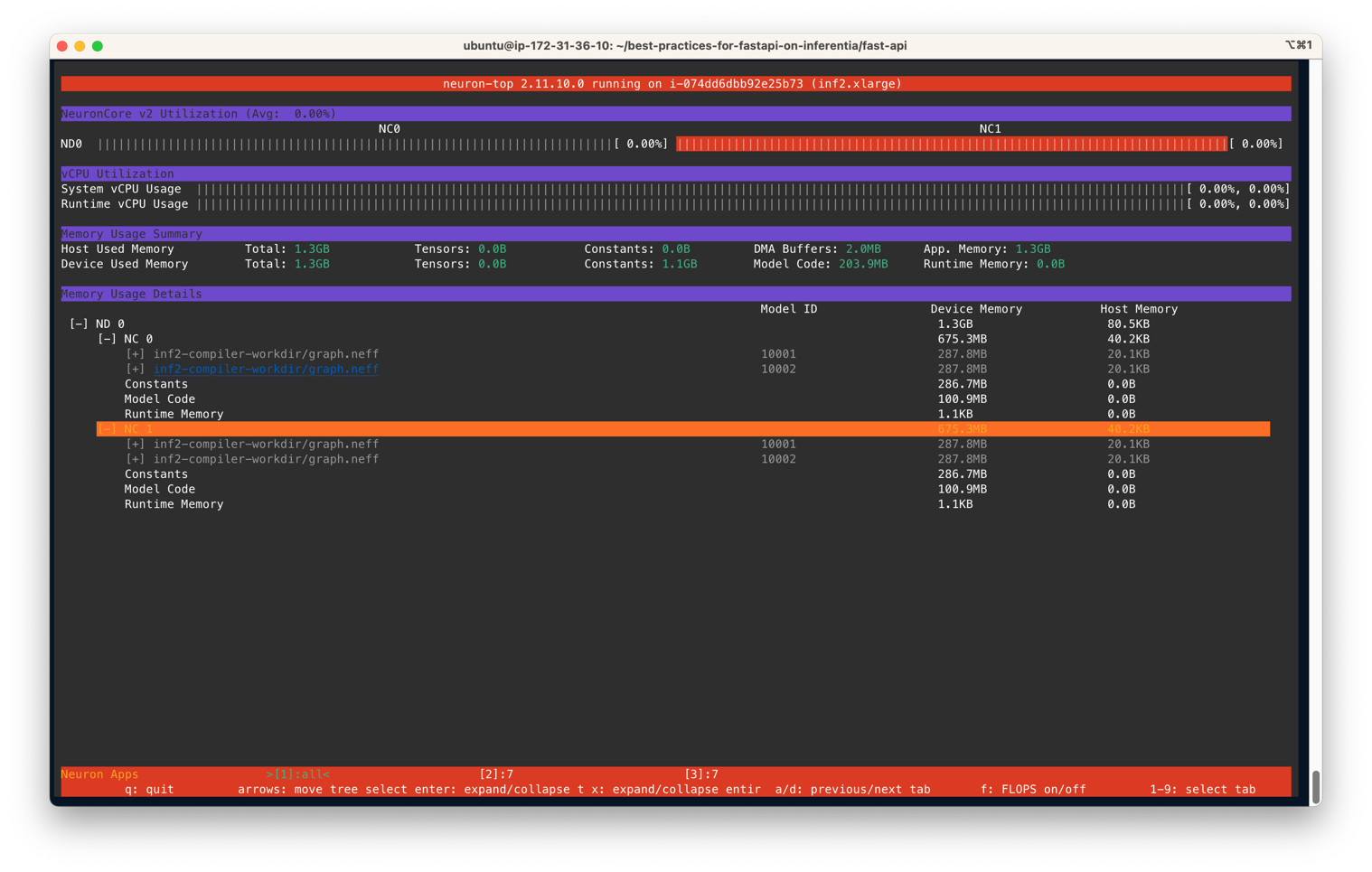
After the model servers are deployed, to monitor NeuronCore utilization, we may use neuron-top to observe in real time the utilization percentage of each NeuronCore. neuron-top is a CLI tool in the Neuron SDK to provide information such as NeuronCore, vCPU, and memory utilization. In a separate terminal, enter the following command:
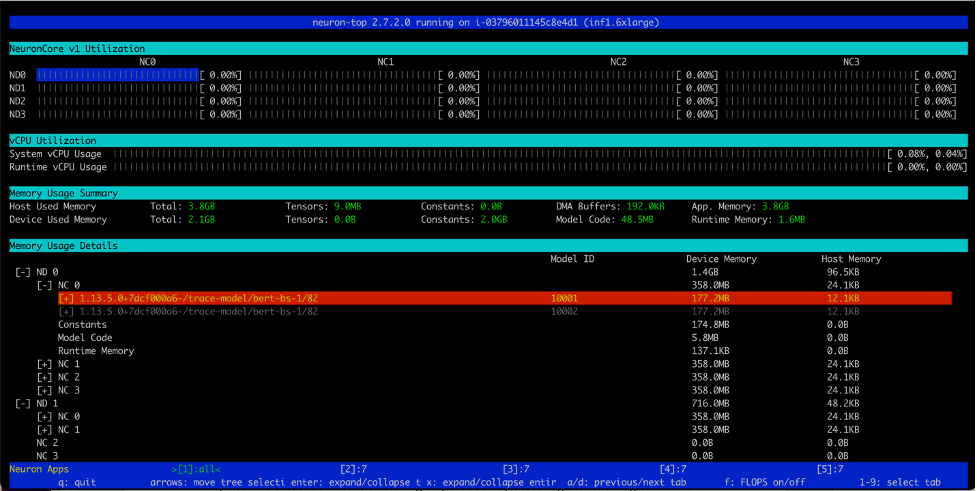
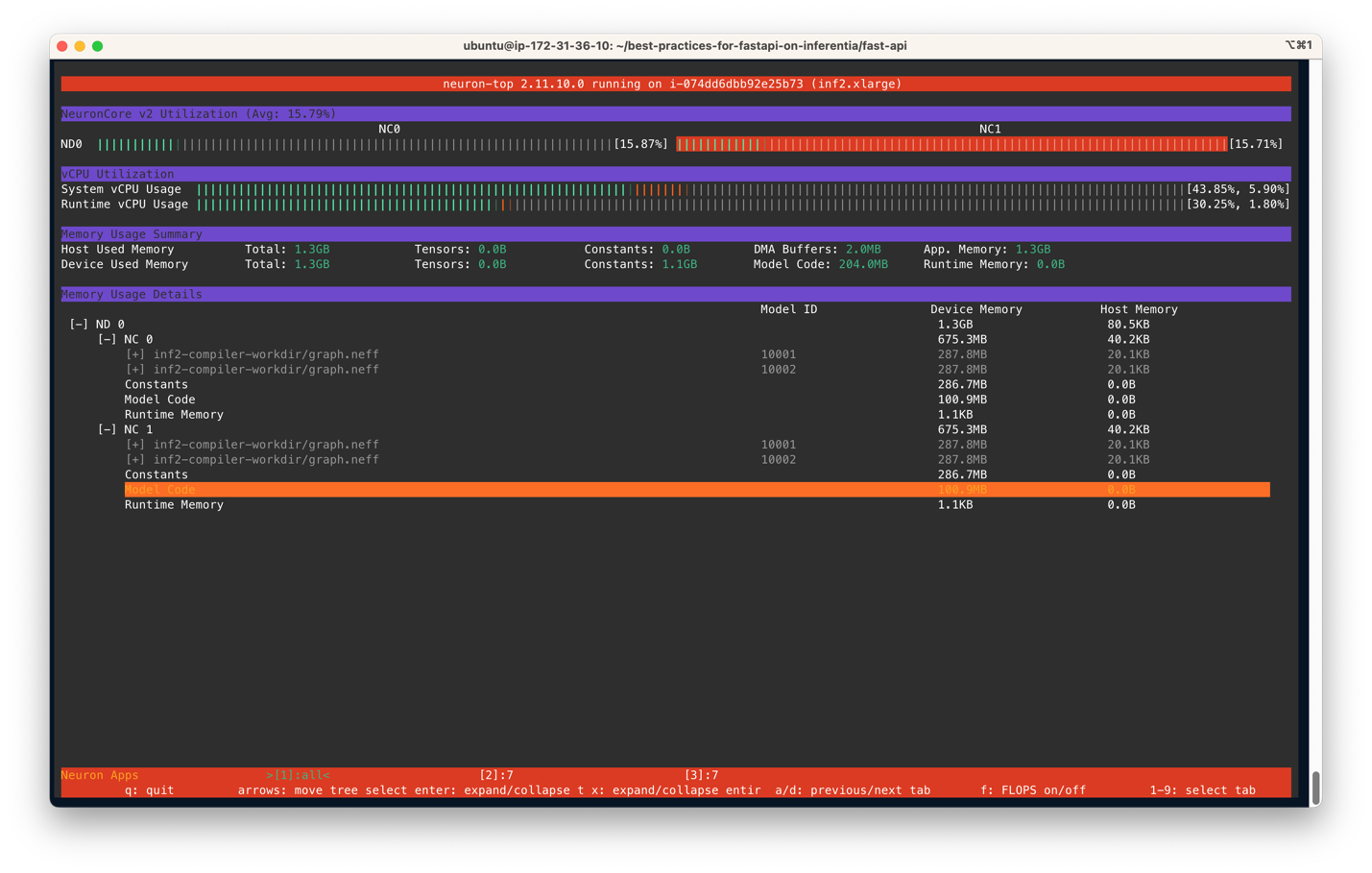
You output should be similar to the following figure. In this scenario, we have specified to use two NeuronCores and two models per server on an Inf2.xlarge instance. The following screenshot shows that two models of size 287.8MB each are loaded on two NeuronCores. With a total of 4 models loaded, you can see the device memory used is 1.3 GB. Use the arrow keys to move between the NeuronCores on different devices
Similarly, on an Inf1.16xlarge instance type we see a total of 12 models (2 models per core over 6 cores) loaded. A total memory of 2.1GB is consumed and every model is 177.2MB in size.
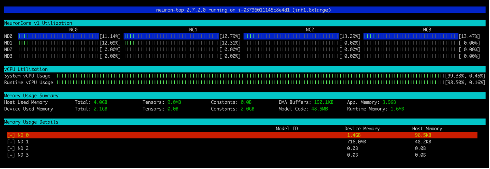
After you run the run_apis.py script, you can see the percentage of utilization of each of the six NeuronCores (see the following screenshot). You can also see the system vCPU usage and runtime vCPU usage.
The following screenshot shows the Inf2 instance core usage percentage.
Similarly, this screenshot shows core utilization in an inf1.6xlarge instance type.
Clean up
To clean up all the Docker containers you created, we provide a cleanup.sh script that removes all running and stopped containers. This script will remove all containers, so don’t use it if you want to keep some containers running.
Conclusion
Production workloads often have high throughput, low latency, and cost requirements. Inefficient architectures that sub-optimally utilize accelerators could lead to unnecessarily high production costs. In this post, we showed how to optimally utilize NeuronCores with FastAPI to maximize throughput at minimum latency. We have published the instructions on our GitHub repo. With this solution architecture, you can deploy multiple models in each NeuronCore and operate multiple models in parallel on different NeuronCores without losing performance. For more information on how to deploy models at scale with services like Amazon Elastic Kubernetes Service (Amazon EKS), refer to Serve 3,000 deep learning models on Amazon EKS with AWS Inferentia for under $50 an hour.
About the authors
 Ankur Srivastava is a Sr. Solutions Architect in the ML Frameworks Team. He focuses on helping customers with self-managed distributed training and inference at scale on AWS. His experience includes industrial predictive maintenance, digital twins, probabilistic design optimization and has completed his doctoral studies from Mechanical Engineering at Rice University and post-doctoral research from Massachusetts Institute of Technology.
 K.C. Tung is a Senior Solution Architect in AWS Annapurna Labs. He specializes in large deep learning model training and deployment at scale in cloud. He has a Ph.D. in molecular biophysics from the University of Texas Southwestern Medical Center in Dallas. He has spoken at AWS Summits and AWS Reinvent. Today he helps customers to train and deploy large PyTorch and TensorFlow models in AWS cloud. He is the author of two books: Learn TensorFlow Enterprise and TensorFlow 2 Pocket Reference.
 Pronoy Chopra is a Senior Solutions Architect with the Startups Generative AI team at AWS. He specializes in architecting and developing IoT and Machine Learning solutions. He has co-founded two startups in the past and enjoys being hands-on with projects in the IoT, AI/ML and Serverless domain.