As machine learning (ML) goes mainstream and gains wider adoption, ML-powered inference applications are becoming increasingly common to solve a range of complex business problems. The solution to these complex business problems often requires using multiple ML models and steps. This post shows you how to build and host an ML application with custom containers on Amazon SageMaker.
Amazon SageMaker offers built-in algorithms and pre-built SageMaker docker images for model deployment. But, if these don’t fit your needs, you can bring your own containers (BYOC) for hosting on Amazon SageMaker.
There are several use cases where users might need to BYOC for hosting on Amazon SageMaker.
- Custom ML frameworks or libraries: If you plan on using a ML framework or libraries that aren’t supported by Amazon SageMaker built-in algorithms or pre-built containers, then you’ll need to create a custom container.
- Specialized models: For certain domains or industries, you may require specific model architectures or tailored preprocessing steps that aren’t available in built-in Amazon SageMaker offerings.
- Proprietary algorithms: If you’ve developed your own proprietary algorithms inhouse, then you’ll need a custom container to deploy them on Amazon SageMaker.
- Complex inference pipelines: If your ML inference workflow involves custom business logic — a series of complex steps that need to be executed in a particular order — then BYOC can help you manage and orchestrate these steps more efficiently.
Solution overview
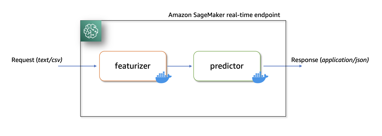
In this solution, we show how to host a ML serial inference application on Amazon SageMaker with real-time endpoints using two custom inference containers with latest scikit-learn and xgboost packages.
The first container uses a scikit-learn model to transform raw data into featurized columns. It applies StandardScaler for numerical columns and OneHotEncoder to categorical ones.

The second container hosts a pretrained XGboost model (i.e., predictor). The predictor model accepts the featurized input and outputs predictions.
Lastly, we deploy the featurizer and predictor in a serial-inference pipeline to an Amazon SageMaker real-time endpoint.
Here are few different considerations as to why you may want to have separate containers within your inference application.
- Decoupling – Various steps of the pipeline have a clearly defined purpose and need to be run on separate containers due to the underlying dependencies involved. This also helps keep the pipeline well structured.
- Frameworks – Various steps of the pipeline use specific fit-for-purpose frameworks (such as scikit or Spark ML) and therefore need to be run on separate containers.
- Resource isolation – Various steps of the pipeline have varying resource consumption requirements and therefore need to be run on separate containers for more flexibility and control.
- Maintenance and upgrades – From an operational standpoint, this promotes functional isolation and you can continue to upgrade or modify individual steps much more easily, without affecting other models.
Additionally, local build of the individual containers helps in the iterative process of development and testing with favorite tools and Integrated Development Environments (IDEs). Once the containers are ready, you can use deploy them to the AWS cloud for inference using Amazon SageMaker endpoints.
Full implementation, including code snippets, is available in this Github repository here.
Prerequisites
As we test these custom containers locally first, we’ll need docker desktop installed on your local computer. You should be familiar with building docker containers.
You’ll also need an AWS account with access to Amazon SageMaker, Amazon ECR and Amazon S3 to test this application end-to-end.
Ensure you have the latest version of Boto3 and the Amazon SageMaker Python packages installed:
pip install --upgrade boto3 sagemaker scikit-learn
Solution Walkthrough
Build custom featurizer container
To build the first container, the featurizer container, we train a scikit-learn model to process raw features in the abalone dataset. The preprocessing script uses SimpleImputer for handling missing values, StandardScaler for normalizing numerical columns, and OneHotEncoder for transforming categorical columns. After fitting the transformer, we save the model in joblib format. We then compress and upload this saved model artifact to an Amazon Simple Storage Service (Amazon S3) bucket.
Here’s a sample code snippet that demonstrates this. Refer to featurizer.ipynb for full implementation:
```python
numeric_features = list(feature_columns_names)
numeric_features.remove("sex")
numeric_transformer = Pipeline(
    steps=[
        ("imputer", SimpleImputer(strategy="median")),
        ("scaler", StandardScaler()),
    ]
)

categorical_features = ["sex"]
categorical_transformer = Pipeline(
    steps=[
        ("imputer", SimpleImputer(strategy="constant", fill_value="missing")),
        ("onehot", OneHotEncoder(handle_unknown="ignore")),
    ]
)

preprocess = ColumnTransformer(
    transformers=[
        ("num", numeric_transformer, numeric_features),
        ("cat", categorical_transformer, categorical_features),
    ]
)

# Call fit on ColumnTransformer to fit all transformers to X, y
preprocessor = preprocess.fit(df_train_val)

# Save the processor model to disk
joblib.dump(preprocess, os.path.join(model_dir, "preprocess.joblib"))
```
Next, to create a custom inference container for the featurizer model, we build a Docker image with nginx, gunicorn, flask packages, along with other required dependencies for the featurizer model.
Nginx, gunicorn and the Flask app will serve as the model serving stack on Amazon SageMaker real-time endpoints.
When bringing custom containers for hosting on Amazon SageMaker, we need to ensure that the inference script performs the following tasks after being launched inside the container:
- Model loading: Inference script (
preprocessing.py) should refer to /opt/ml/model directory to load the model in the container. Model artifacts in Amazon S3 will be downloaded and mounted onto the container at the path /opt/ml/model.
- Environment variables: To pass custom environment variables to the container, you must specify them during the Model creation step or during Endpoint creation from a training job.
- API requirements: The Inference script must implement both
/ping and /invocations routes as a Flask application. The /ping API is used for health checks, while the /invocations API handles inference requests.
- Logging: Output logs in the inference script must be written to standard output (stdout) and standard error (stderr) streams. These logs are then streamed to Amazon CloudWatch by Amazon SageMaker.
Here’s a snippet from preprocessing.py that show the implementation of /ping and /invocations.
Refer to preprocessing.py under the featurizer folder for full implementation.
```python
def load_model():
    # Construct the path to the featurizer model file
    ft_model_path = os.path.join(MODEL_PATH, "preprocess.joblib")
    featurizer = None

    try:
        # Open the model file and load the featurizer using joblib
        with open(ft_model_path, "rb") as f:
            featurizer = joblib.load(f)
            print("Featurizer model loaded", flush=True)
    except FileNotFoundError:
        print(f"Error: Featurizer model file not found at {ft_model_path}", flush=True)
    except Exception as e:
        print(f"Error loading featurizer model: {e}", flush=True)

    # Return the loaded featurizer model, or None if there was an error
    return featurizer

def transform_fn(request_body, request_content_type):
    """
    Transform the request body into a usable numpy array for the model.

    This function takes the request body and content type as input, and
    returns a transformed numpy array that can be used as input for the
    prediction model.

    Parameters:
        request_body (str): The request body containing the input data.
        request_content_type (str): The content type of the request body.

    Returns:
        data (np.ndarray): Transformed input data as a numpy array.
    """
    # Define the column names for the input data
    feature_columns_names = [
        "sex",
        "length",
        "diameter",
        "height",
        "whole_weight",
        "shucked_weight",
        "viscera_weight",
        "shell_weight",
    ]
    label_column = "rings"

    # Check if the request content type is supported (text/csv)
    if request_content_type == "text/csv":
        # Load the featurizer model
        featurizer = load_model()

        # Check if the featurizer is a ColumnTransformer
        if isinstance(
            featurizer, sklearn.compose._column_transformer.ColumnTransformer
        ):
            print(f"Featurizer model loaded", flush=True)

        # Read the input data from the request body as a CSV file
        df = pd.read_csv(StringIO(request_body), header=None)

        # Assign column names based on the number of columns in the input data
        if len(df.columns) == len(feature_columns_names) + 1:
            # This is a labelled example, includes the ring label
            df.columns = feature_columns_names + [label_column]
        elif len(df.columns) == len(feature_columns_names):
            # This is an unlabelled example.
            df.columns = feature_columns_names

        # Transform the input data using the featurizer
        data = featurizer.transform(df)

        # Return the transformed data as a numpy array
        return data
    else:
        # Raise an error if the content type is unsupported
        raise ValueError("Unsupported content type: {}".format(request_content_type))


@app.route("/ping", methods=["GET"])
def ping():
    # Check if the model can be loaded, set the status accordingly
    featurizer = load_model()
    status = 200 if featurizer is not None else 500

    # Return the response with the determined status code
    return flask.Response(response="n", status=status, mimetype="application/json")


@app.route("/invocations", methods=["POST"])
def invocations():
    # Convert from JSON to dict
    print(f"Featurizer: received content type: {flask.request.content_type}")
    if flask.request.content_type == "text/csv":
        # Decode input data and transform
        input = flask.request.data.decode("utf-8")
        transformed_data = transform_fn(input, flask.request.content_type)

        # Format transformed_data into a csv string
        csv_buffer = io.StringIO()
        csv_writer = csv.writer(csv_buffer)

        for row in transformed_data:
            csv_writer.writerow(row)

        csv_buffer.seek(0)

        # Return the transformed data as a CSV string in the response
        return flask.Response(response=csv_buffer, status=200, mimetype="text/csv")
    else:
        print(f"Received: {flask.request.content_type}", flush=True)
        return flask.Response(
            response="Transformer: This predictor only supports CSV data",
            status=415,
            mimetype="text/plain",
        )
```
Build Docker image with featurizer and model serving stack
Let’s now build a Dockerfile using a custom base image and install required dependencies.
For this, we use python:3.9-slim-buster as the base image. You can change this any other base image relevant to your use case.
We then copy the nginx configuration, gunicorn’s web server gateway file, and the inference script to the container. We also create a python script called serve that launches nginx and gunicorn processes in the background and sets the inference script (i.e., preprocessing.py Flask application) as the entry point for the container.
Here’s a snippet of the Dockerfile for hosting the featurizer model. For full implementation refer to Dockerfile under featurizer folder.
```docker
FROM python:3.9-slim-buster
…

# Copy requirements.txt to /opt/program folder
COPY requirements.txt /opt/program/requirements.txt

# Install packages listed in requirements.txt
RUN pip3 install --no-cache-dir -r /opt/program/requirements.txt

# Copy contents of code/ dir to /opt/program
COPY code/ /opt/program/

# Set working dir to /opt/program which has the serve and inference.py scripts
WORKDIR /opt/program

# Expose port 8080 for serving
EXPOSE 8080

ENTRYPOINT ["python"]

# serve is a python script under code/ directory that launches nginx and gunicorn processes
CMD [ "serve" ]
```
Test custom inference image with featurizer locally
Now, build and test the custom inference container with featurizer locally, using Amazon SageMaker local mode. Local mode is perfect for testing your processing, training, and inference scripts without launching any jobs on Amazon SageMaker. After confirming the results of your local tests, you can easily adapt the training and inference scripts for deployment on Amazon SageMaker with minimal changes.
To test the featurizer custom image locally, first build the image using the previously defined Dockerfile. Then, launch a container by mounting the directory containing the featurizer model (preprocess.joblib) to the /opt/ml/model directory inside the container. Additionally, map port 8080 from container to the host.
Once launched, you can send inference requests to http://localhost:8080/invocations.
To build and launch the container, open a terminal and run the following commands.
Note that you should replace the <IMAGE_NAME>, as shown in the following code, with the image name of your container.
The following command also assumes that the trained scikit-learn model (preprocess.joblib) is present under a directory called models.
```shell
docker build -t <IMAGE_NAME> .
```

```shell
docker run –rm -v $(pwd)/models:/opt/ml/model -p 8080:8080 <IMAGE_NAME>
```
After the container is up and running, we can test both the /ping and /invocations routes using curl commands.
Run the below commands from a terminal
```shell
# test /ping route on local endpoint
curl http://localhost:8080/ping

# send raw csv string to /invocations. Endpoint should return transformed data
curl --data-raw 'I,0.365,0.295,0.095,0.25,0.1075,0.0545,0.08,9.0' -H 'Content-Type: text/csv' -v http://localhost:8080/invocations
```
When raw (untransformed) data is sent to http://localhost:8080/invocations, the endpoint responds with transformed data.
You should see response something similar to the following:
```shell
* Trying 127.0.0.1:8080...
* Connected to localhost (127.0.0.1) port 8080 (#0)
> POST /invocations HTTP/1.1
> Host: localhost: 8080
> User-Agent: curl/7.87.0
> Accept: */*
> Content -Type: text/csv
> Content -Length: 47
>
* Mark bundle as not supporting multiuse
> HTTP/1.1 200 OK
> Server: nginx/1.14.2
> Date: Sun, 09 Apr 2023 20:47:48 GMT
> Content -Type: text/csv; charset=utf-8
> Content -Length: 150
> Connection: keep -alive
-1.3317586042173168, -1.1425409076053987, -1.0579488602777858, -1.177706547272754, -1.130662184748842,
* Connection #0 to host localhost left intact
```
We now terminate the running container, and then tag and push the local custom image to a private Amazon Elastic Container Registry (Amazon ECR) repository.
See the following commands to login to Amazon ECR, which tags the local image with full Amazon ECR image path and then push the image to Amazon ECR. Ensure you replace region and account variables to match your environment.
```shell
# login to ecr with your credentials
aws ecr get-login-password - -region "${region}" |
docker login - -username AWS - -password-stdin ${account}".dkr.ecr."${region}".amazonaws.com

# tag and push the image to private Amazon ECR
docker tag ${image} ${fullname}
docker push $ {fullname}

```
Refer to create a repository and push an image to Amazon ECR AWS Command Line Interface (AWS CLI) commands for more information.
Optional step
Optionally, you could perform a live test by deploying the featurizer model to a real-time endpoint with the custom docker image in Amazon ECR. Refer to featurizer.ipynb notebook for full implementation of buiding, testing, and pushing the custom image to Amazon ECR.
Amazon SageMaker initializes the inference endpoint and copies the model artifacts to the /opt/ml/model directory inside the container. See How SageMaker Loads your Model artifacts.
Build custom XGBoost predictor container
For building the XGBoost inference container we follow similar steps as we did while building the image for featurizer container:
- Download pre-trained
XGBoost model from Amazon S3.
- Create the
inference.py script that loads the pretrained XGBoost model, converts the transformed input data received from featurizer, and converts to XGBoost.DMatrix format, runs predict on the booster, and returns predictions in json format.
- Scripts and configuration files that form the model serving stack (i.e.,
nginx.conf, wsgi.py, and serve remain the same and needs no modification.
- We use
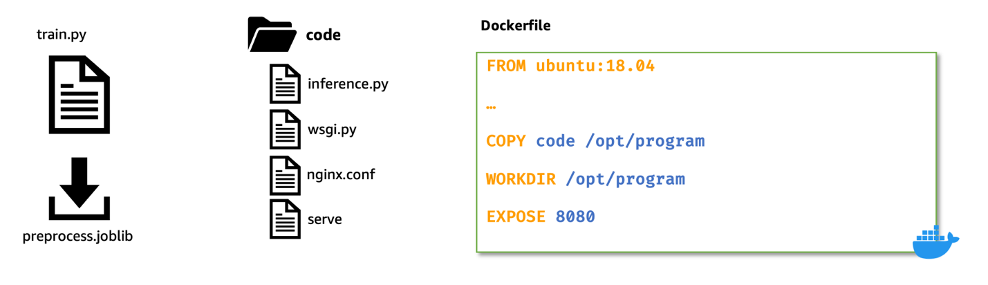
Ubuntu:18.04 as the base image for the Dockerfile. This isn’t a prerequisite. We use the ubuntu base image to demonstrate that containers can be built with any base image.
- The steps for building the customer docker image, testing the image locally, and pushing the tested image to Amazon ECR remain the same as before.
For brevity, as the steps are similar shown previously; however, we only show the changed coding in the following.
First, the inference.py script. Here’s a snippet that show the implementation of /ping and /invocations. Refer to inference.py under the predictor folder for full implementation of this file.
```python
@app.route("/ping", methods=["GET"])
def ping():
    """
    Check the health of the model server by verifying if the model is loaded.

    Returns a 200 status code if the model is loaded successfully, or a 500
    status code if there is an error.

    Returns:
        flask.Response: A response object containing the status code and mimetype.
    """
    status = 200 if model is not None else 500
    return flask.Response(response="n", status=status, mimetype="application/json")

@app.route("/invocations", methods=["POST"])
def invocations():
    """
    Handle prediction requests by preprocessing the input data, making predictions,
    and returning the predictions as a JSON object.

    This function checks if the request content type is supported (text/csv; charset=utf-8),
    and if so, decodes the input data, preprocesses it, makes predictions, and returns
    the predictions as a JSON object. If the content type is not supported, a 415 status
    code is returned.

    Returns:
        flask.Response: A response object containing the predictions, status code, and mimetype.
    """
    print(f"Predictor: received content type: {flask.request.content_type}")
    if flask.request.content_type == "text/csv; charset=utf-8":
        input = flask.request.data.decode("utf-8")
        transformed_data = preprocess(input, flask.request.content_type)
        predictions = predict(transformed_data)

        # Return the predictions as a JSON object
        return json.dumps({"result": predictions})
    else:
        print(f"Received: {flask.request.content_type}", flush=True)
        return flask.Response(
            response=f"XGBPredictor: This predictor only supports CSV data; Received: {flask.request.content_type}",
            status=415,
            mimetype="text/plain",
        )

```
Here’s a snippet of the Dockerfile for hosting the predictor model. For full implementation refer to Dockerfile under predictor folder.
```docker
FROM ubuntu:18.04

…

# install required dependencies including flask, gunicorn, xgboost etc.,
RUN pip3 --no-cache-dir install  flask  gunicorn  gevent  numpy  pandas  xgboost

# Copy contents of code/ dir to /opt/program
COPY code /opt/program

# Set working dir to /opt/program which has the serve and inference.py scripts
WORKDIR /opt/program

# Expose port 8080 for serving
EXPOSE 8080

ENTRYPOINT ["python"]

# serve is a python script under code/ directory that launches nginx and gunicorn processes
CMD ["serve"]
```
We then continue to build, test, and push this custom predictor image to a private repository in Amazon ECR. Refer to predictor.ipynb notebook for full implementation of building, testing and pushing the custom image to Amazon ECR.
Deploy serial inference pipeline
After we have tested both the featurizer and predictor images and have pushed them to Amazon ECR, we now upload our model artifacts to an Amazon S3 bucket.
Then, we create two model objects: one for the featurizer (i.e., preprocess.joblib) and other for the predictor (i.e., xgboost-model) by specifying the custom image uri we built earlier.
Here’s a snippet that shows that. Refer to serial-inference-pipeline.ipynb for full implementation.
```python
suffix = f"{str(uuid4())[:5]}-{datetime.now().strftime('%d%b%Y')}"

# Featurizer Model (SKLearn Model)
image_name = "<FEATURIZER_IMAGE_NAME>"
sklearn_image_uri = f"{account_id}.dkr.ecr.{region}.amazonaws.com/{image_name}:latest"

featurizer_model_name = f""<FEATURIZER_MODEL_NAME>-{suffix}"
print(f"Creating Featurizer model: {featurizer_model_name}")
sklearn_model = Model(
    image_uri=featurizer_ecr_repo_uri,
    name=featurizer_model_name,
    model_data=featurizer_model_data,
    role=role,
)

# Full name of the ECR repository
predictor_image_name = "<PREDICTOR_IMAGE_NAME>"
predictor_ecr_repo_uri
= f"{account_id}.dkr.ecr.{region}.amazonaws.com/{predictor_image_name}:latest"

# Predictor Model (XGBoost Model)
predictor_model_name = f"""<PREDICTOR_MODEL_NAME>-{suffix}"
print(f"Creating Predictor model: {predictor_model_name}")
xgboost_model = Model(
    image_uri=predictor_ecr_repo_uri,
    name=predictor_model_name,
    model_data=predictor_model_data,
    role=role,
)
```
Now, to deploy these containers in a serial fashion, we first create a PipelineModel object and pass the featurizer model and the predictor model to a python list object in the same order.
Then, we call the .deploy() method on the PipelineModel specifying the instance type and instance count.
```python
from sagemaker.pipeline import PipelineModel

pipeline_model_name = f"Abalone-pipeline-{suffix}"

pipeline_model = PipelineModel(
    name=pipeline_model_name,
    role=role,
    models=[sklearn_model, xgboost_model],
    sagemaker_session=sm_session,
)

print(f"Deploying pipeline model {pipeline_model_name}...")
predictor = pipeline_model.deploy(
    initial_instance_count=1,
    instance_type="ml.m5.xlarge",
)
```
At this stage, Amazon SageMaker deploys the serial inference pipeline to a real-time endpoint. We wait for the endpoint to be InService.
We can now test the endpoint by sending some inference requests to this live endpoint.
Refer to serial-inference-pipeline.ipynb for full implementation.
Clean up
After you are done testing, please follow the instructions in the cleanup section of the notebook to delete the resources provisioned in this post to avoid unnecessary charges. Refer to Amazon SageMaker Pricing for details on the cost of the inference instances.
```python
# Delete endpoint, model
try:
    print(f"Deleting model: {pipeline_model_name}")
    predictor.delete_model()
except Exception as e:
    print(f"Error deleting model: {pipeline_model_name}n{e}")
    pass

try:
    print(f"Deleting endpoint: {endpoint_name}")
    predictor.delete_endpoint()
except Exception as e:
    print(f"Error deleting EP: {endpoint_name}n{e}")
    pass

```
Conclusion
In this post, I showed how we can build and deploy a serial ML inference application using custom inference containers to real-time endpoints on Amazon SageMaker.
This solution demonstrates how customers can bring their own custom containers for hosting on Amazon SageMaker in a cost-efficient manner. With BYOC option, customers can quickly build and adapt their ML applications to be deployed on to Amazon SageMaker.
We encourage you to try this solution with a dataset relevant to your business Key Performance Indicators (KPIs). You can refer to the entire solution in this GitHub repository.
References
About the Author
 Praveen Chamarthi is a Senior AI/ML Specialist with Amazon Web Services. He is passionate about AI/ML and all things AWS. He helps customers across the Americas to scale, innovate, and operate ML workloads efficiently on AWS. In his spare time, Praveen loves to read and enjoys sci-fi movies.
Read More
 The contest is open to anyone with a creative and innovative idea that could impact the world. The only catch? The idea must originate — like NVIDIA — in a Denny’s booth.
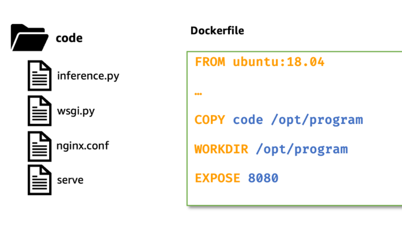

 A round-up of our top 10 AI moments of the last 25 years.


 Jun Zhang is a Solutions Architect based in Zurich. He helps Swiss customers architect cloud-based solutions to achieve their business potential. He has a passion for sustainability and strives to solve current sustainability challenges with technology. He is also a huge tennis fan and enjoys playing board games a lot.
 Mohan Gowda leads Machine Learning team at AWS Switzerland. He works primarily with Automotive customers to develop innovative AI/ML solutions and platforms for next generation vehicles. Before working with AWS, Mohan worked with a Global Management Consulting firm with a focus on Strategy & Analytics. His passion lies in connected vehicles and autonomous driving.
 Matthias Egli is the Head of Education in Switzerland. He is an enthusiastic Team Lead with a broad experience in business development, sales, and marketing.
 Kemeng Zhang is an ML Engineer based in Zurich. She helps global customers design, develop, and scale ML-based applications to empower their digital capabilities to increase business revenue and reduce cost. She is also very passionate about creating human-centric applications by leveraging knowledge from behavioral science. She likes playing water sports and walking dogs.
 Daniele Chiappalupi is a recent graduate from ETH Zürich. He enjoys every aspect of software engineering, from design to implementation, and from deployment to maintenance. He has a deep passion for AI and eagerly anticipates exploring, utilizing, and contributing to the latest advancements in the field. In his free time, he loves going snowboarding during colder months and playing pick-up basketball when the weather warms up.


 Gagan Singh is a Senior Technical Account Manager at AWS, where he partners with digital native startups to pave their path to heightened business success. With a niche in propelling Machine Learning initiatives, he leverages Amazon SageMaker, particularly emphasizing on Deep Learning and Generative AI solutions. In his free time, Gagan finds solace in trekking on the trails of the Himalayas and immersing himself in diverse music genres.
 Dhawal Patel is a Principal Machine Learning Architect at AWS. He has worked with organizations ranging from large enterprises to mid-sized startups on problems related to distributed computing, and Artificial Intelligence. He focuses on Deep learning including NLP and Computer Vision domains. He helps customers achieve high performance model inference on SageMaker.
 Venugopal Pai is a Solutions Architect at AWS. He lives in Bengaluru, India, and helps digital native customers scale and optimize their applications on AWS.