Monthly Archives: September 2023

Use 3D to visualize matrix multiplication expressions, attention heads with real weights, and more.

Matrix multiplications (matmuls) are the building blocks of today’s ML models. This note presents mm, a visualization tool for matmuls and compositions of matmuls.

Because mm uses all three spatial dimensions, it helps build intuition and spark ideas with less cognitive overhead than the usual squares-on-paper idioms, especially (though not only) for visual/spatial thinkers.

And with three dimensions available for composing matmuls, along with the ability to load trained weights, we can visualize big, compound expressions like attention heads and observe how they actually behave, using im.

mm is fully interactive, runs in the browser or notebook iframes and keeps its complete state in the URL, so links are shareable sessions (the screenshots and videos in this note all have links that open the visualizations in the tool). This reference guide describes all of the available functionality.

We’ll first introduce the visualization approach, build intuition by visualizing some simple matmuls and expressions, then dive into some more extended examples:

1. Pitch – why is this way of visualizing better?
2. Warmup – animations – watching the canonical matmul decompositions in action
3. Warmup – expressions – a quick tour of some fundamental expression building blocks
4. Inside an attention head – an in-depth look at the structure, values and computation behavior of a couple of attention heads from GPT2 via NanoGPT
5. Parallelizing attention – visualizing attention head parallelization with examples from the recent Blockwise Parallel Transformer paper
6. Sizes in an attention layer – what do the MHA and FFA halves of an attention layer look like together, when we visualize a whole layer as a single structure? How does the picture change during autoregressive decoding?
7. LoRA – a visual explanation of this elaboration of the attention head architecture
8. Wrapup – next steps and call for feedback

1 Pitch

mm’s visualization approach is based on the premise that matrix multiplication is fundamentally a three-dimensional operation.

In other words this:

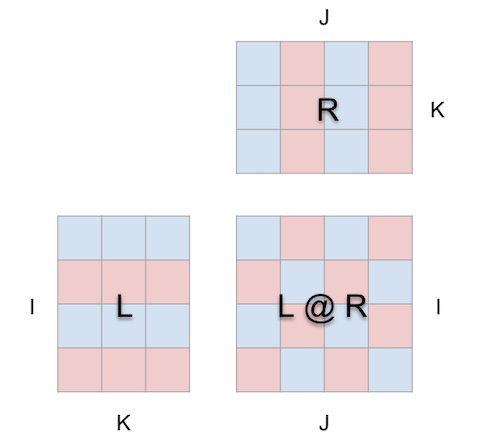
is a sheet of paper trying to be this (open in mm):

When we wrap the matmul around a cube this way, the correct relationships between argument shapes, result shape and shared dimensions all fall into place.

Now the computation makes geometric sense: each location i, j in the result matrix anchors a vector running along the depth dimension k in the cube’s interior, where the horizontal plane extending from row i in L and a vertical plane extending from column j in R intersect. Along this vector, pairs of (i, k) (k, j) elements from the left and right arguments meet and are multiplied, and the resulting products are summed along k and the result is deposited in location i, j of the result.

(Jumping ahead momentarily, here’s an animation.)

This is the intuitive meaning of matrix multiplication:

1. project two orthogonal matrices into the interior of a cube
2. multiply the pair of values at each intersection, forming a grid of products
3. sum along the third orthogonal dimension to produce a result matrix.

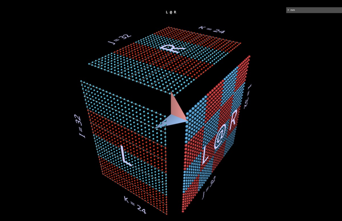
For orientation, the tool displays an arrow in the cube’s interior that points towards the result matrix, with a blue vane coming from the left argument and a red vane coming from the right argument. The tool also displays white guidelines to indicate the row axis of each matrix, though they’re faint in this screenshot.

The layout constraints are straightforward:

• left argument and result must be adjoined along their shared height (i) dimension
• right argument and result must be adjoined along their shared width (j) dimension
• left and right arguments must be adjoined along their shared (left width/right height) dimension, which becomes the matmul’s depth (k) dimension

This geometry gives us a solid foundation for visualizing all the standard matmul decompositions, and an intuitive basis for exploring nontrivially complex compositions of matmuls, as we’ll see below.

2 Warmup – animations

Before diving into some more complex examples, we’ll run through a few intuition builders to get a feel for how things look and feel in this style of visualization.

2a Dot product

First, the canonical algorithm – computing each result element by taking the dot product of the corresponding left row and right column. What we see in the animation is the sweep of multiplied value vectors through the cube’s interior, each delivering a summed result at the corresponding position.

Here, L has blocks of rows filled with 1 (blue) or -1 (red); R has column blocks filled similarly. k is 24 here, so the result matrix (L @ R) has blue values of 24 and red values of -24 (open in mm – long click or control-click to inspect values):

2b Matrix-vector products

A matmul decomposed into matrix-vector products looks like a vertical plane (a product of the left argument with each column of the right argument) painting columns onto the result as it sweeps horizontally through the cube’s interior (open in mm):

Observing the intermediate values of a decomposition can be quite interesting, even in simple examples.

For instance, note the prominent vertical patterns in the intermediate matrix-vector products when we use randomly initialized arguments- reflecting the fact that each intermediate is a column-scaled replica of the left argument (open in mm):

2c Vector-matrix products

A matmul decomposed into vector-matrix products looks like a horizontal plane painting rows onto the result as it descends through the cube’s interior (open in mm):

Switching to randomly initialized arguments, we see patterns analogous to those we saw with matrix-vector products – only this time the patterns are horizontal, corresponding to the fact that each intermediate vector-matrix product is a row-scaled replica of the right argument.

When thinking about how matmuls express the rank and structure of their arguments, it’s useful to envision both of these patterns happening simultaneously in the computation (open in mm):

Here’s one more intuition builder using vector-matrix products, showing how the identity matrix functions exactly like a mirror set at a 45deg angle to both its counterargument and the result (open in mm):

2d Summed outer products

The third planar decomposition is along the k axis, computing the matmul result by a pointwise summation of vector outer products. Here we see the plane of outer products sweeping the cube “from back to front”, accumulating into the result (open in mm):

Using randomly initialized matrices with this decomposition, we can see not just values but rank accumulate in the result, as each rank-1 outer product is added to it.

Among other things this builds intuition for why “low-rank factorization” – i.e. approximating a matrix by constructing a matmul whose arguments are small in the depth dimension – works best when the matrix being approximated is low rank. LoRA in a later section (open in mm):

3 Warmup – expressions

How can we extend this visualization approach to compositions of matmuls? Our examples so far have all visualized a single matmul L @ R of some matrices L and R – what about when L and/or R are themselves matmuls, and so on transitively?

It turns out we can extend the approach nicely to compound expressions. The key rules are simple: the subexpression (child) matmul is another cube, subject to the same layout constraints as the parent, and the result face of the child is simultaneously the corresponding argument face of the parent, like a covalently shared electron.

Within these constraints, we’re free to arrange the faces of a child matmul however we like. Here we use the tool’s default scheme, which generates alternating convex and concave cubes – this layout works well in practice to maximize use of space and minimize occlusion. (Layouts are completely customizable, however – see the reference for details.)

In this section we’ll visualize some of the key building blocks we find in ML models, to gain fluency in the visual idiom and to see what intuitions even simple examples can give us.

3a Left-associative expressions

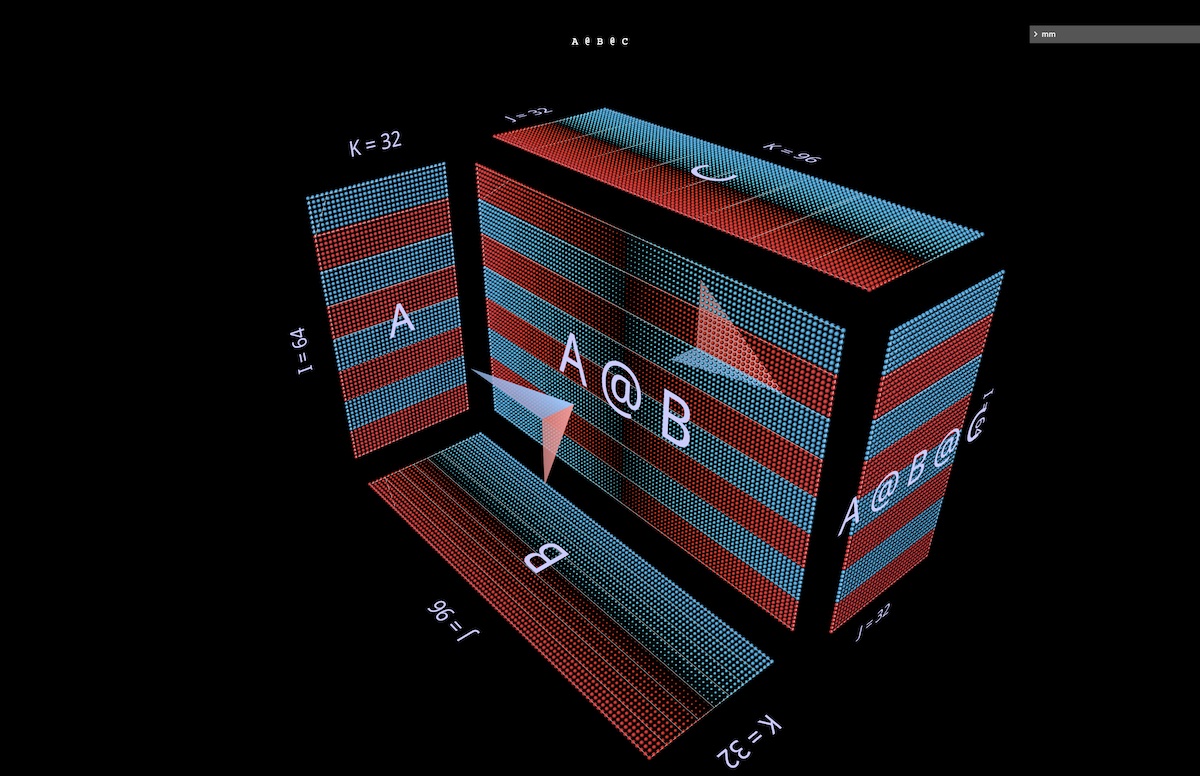
We’ll look at two expressions of the form (A @ B) @ C, each with its own distinctive shape and character. (Note: mm adheres to the convention that matrix multiplication is left-associative and writes this simply as A @ B @ C.)

First we’ll give A @ B @ C the characteristic FFN shape, in which the “hidden dimension” is wider than the “input” or “output” dimensions. (Concretely in the context of this example, this means that the width of B is greater than the widths of A or C.)

As in the single matmul examples, the floating arrows point towards the result matrix, blue vane coming from the left argument and red vane from right argument (open in mm):

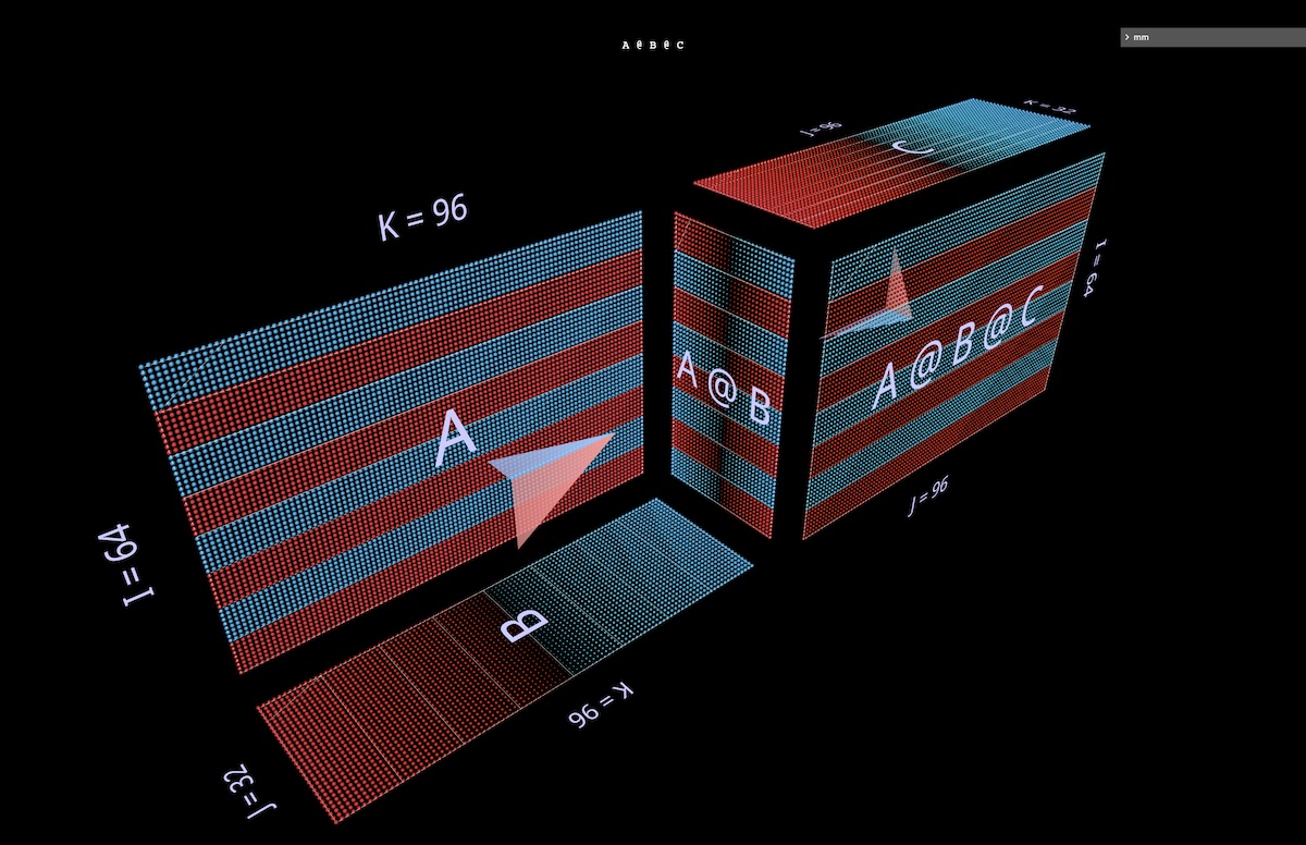
Next we’ll visualize A @ B @ C with the width of B narrower than that of A or C, giving it a bottleneck or “autoencoder” shape (open in mm):

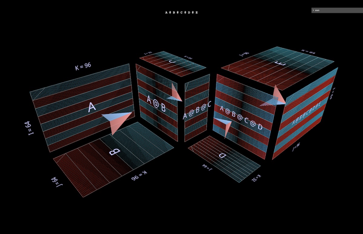
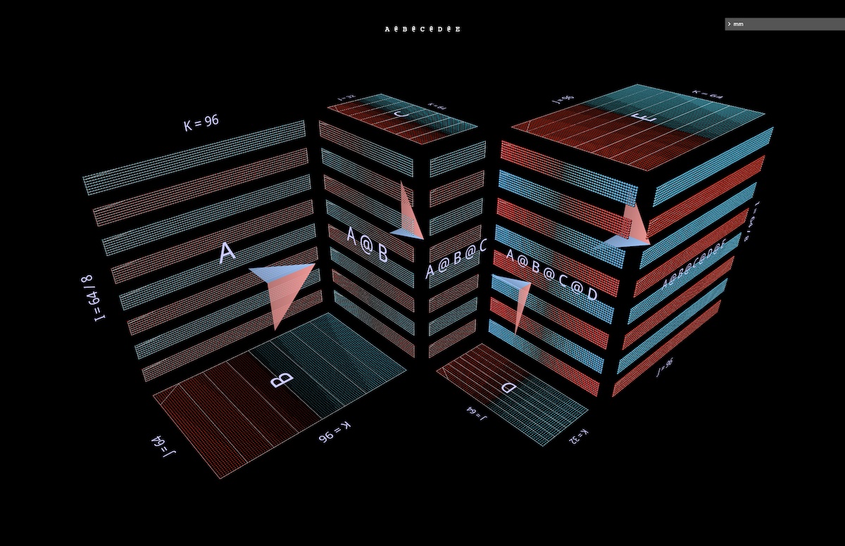
This pattern of alternating convex and concave blocks extends to chains of arbitrary length: for example this multilayer bottleneck (open in mm):

3b Right associative expressions

Next we’ll visualize a right-associative expression A @ (B @ C).

In the same way left-associative expressions extend horizontally – sprouting from the left argument of the root expression, so to speak – right-associative chains extend vertically, sprouting from the root’s right argument.

One sometimes sees an MLP formulated right-associatively, i.e. with columnar input on the right and weight layers running right to left. Using the matrices from the 2-layer FFN example pictured above – suitably transposed – here’s what that looks like, with C now playing the role of the input, B the first layer and A the second layer (open in mm):

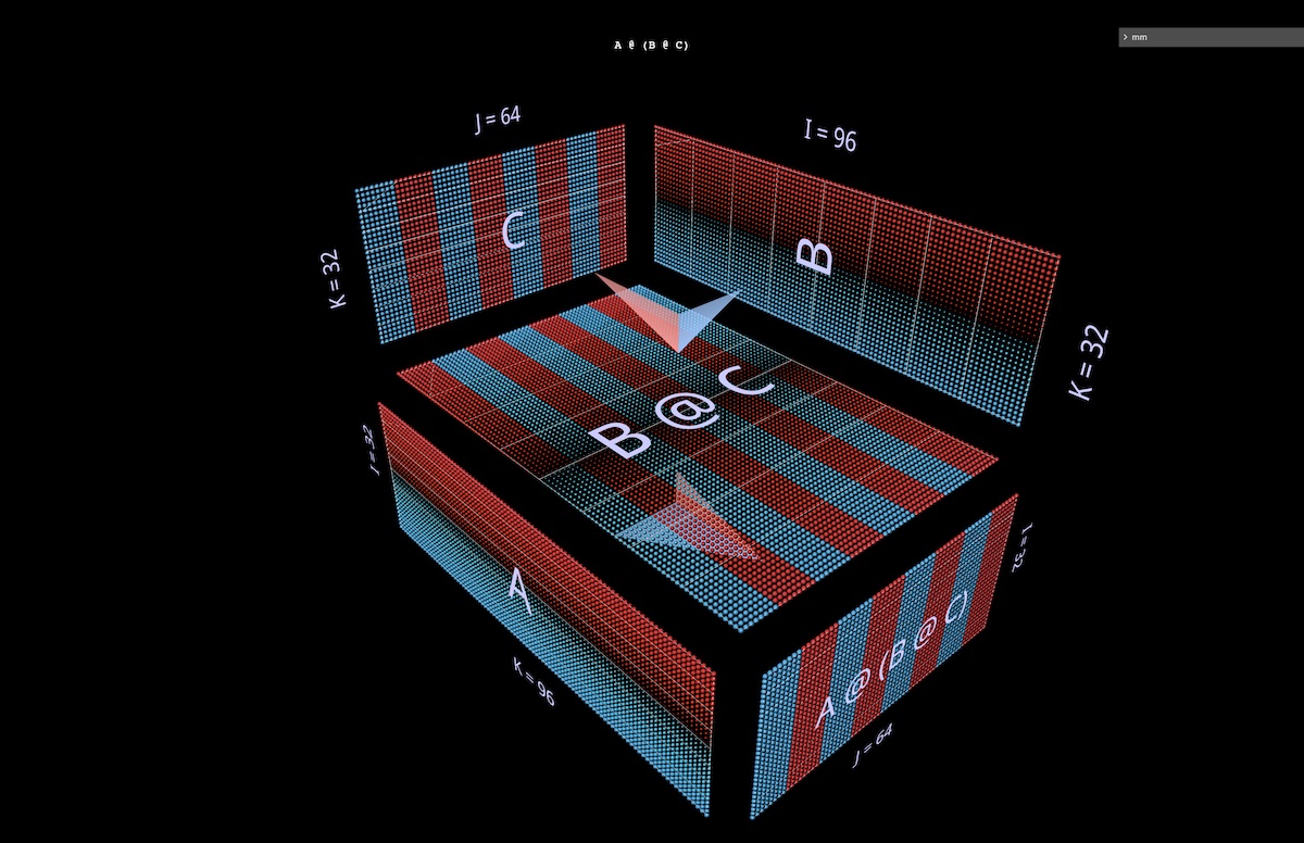
Aside: in addition to the color of the arrow vanes (blue for left, red for right), a second visual cue for distinguishing left and right arguments is their orientation: the rows of the left argument are coplanar with those of the result – they stack along the same axis (i). Both cues tell us for example that B is the left argument to (B @ C) above.

3c Binary expressions

For a visualization tool to be useful beyond simple didactic examples, visualizations need to remain legible as expressions get more complicated. A key structural component in real-world use cases is binary expressions – matmuls with subexpressions on both the left and right.

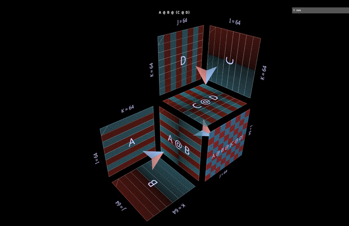
Here we’ll visualize the simplest such expression shape, (A @ B) @ (C @ D) (open in mm):

3d Quick aside: partitioning and parallelism

A full presentation of this topic is out of scope for this note, though we’ll see it in action later in the context of attention heads. But as a warmup, two quick examples should give a sense of how this style of visualization makes reasoning about parallelizing compound expressions very intuitive, via the simple geometry of partitioning.

In the first example we’ll apply the canonical “data parallel” partitioning to the left-associative multilayer bottleneck example above. We partition along i, segmenting the initial left argument (“batch”) and all intermediate results (“activations”), but none of the subsequent arguments (“weights”) – the geometry making it obvious which participants in the expression are segmented and which remain whole (open in mm):

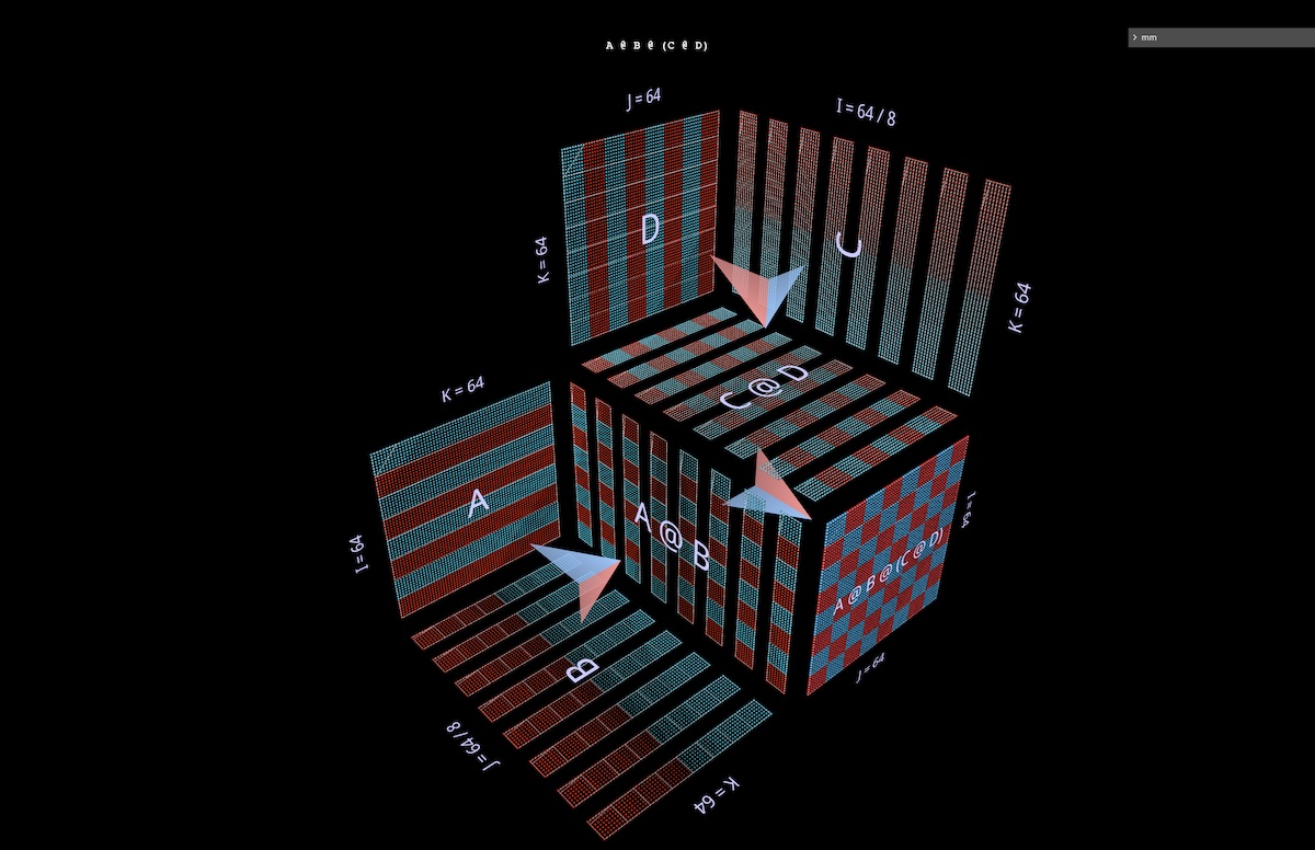
The second example would (for me, anyway) be much harder to build intuition about without clear geometry to support it: it shows how a binary expression can be parallelized by partitioning the left subexpression along its j axis, the right subexpression along its i axis, and the parent expression along its k axis (open in mm):

4 Inside an Attention Head

Let’s look at a GPT2 attention head – specifically layer 5, head 4 of the “gpt2” (small) configuration (layers=12, heads=12, embed=768) from NanoGPT, using OpenAI weights via HuggingFace. Input activations are taken from a forward pass on an OpenWebText training sample of 256 tokens.

There’s nothing particularly unusual about this particular head; I chose it mainly because it computes a fairly common attention pattern and lives in the middle of the model, where activations have become structured and show some interesting texture. (Aside: in a subsequent note I’ll present an attention head explorer that lets you visualize all layers and heads of this model, along with some travel notes.)

Open in mm (may take a few seconds to fetch model weights)

4a Structure

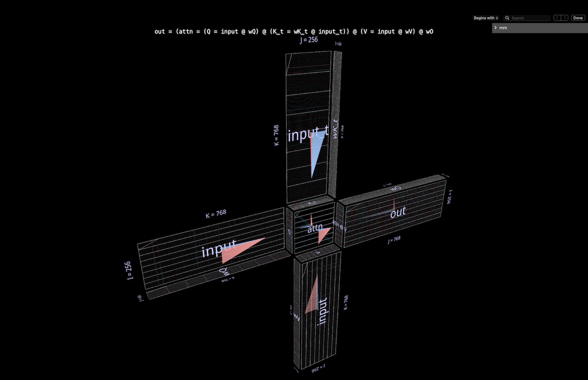
The entire attention head is visualized as a single compound expression, starting with input and ending with projected output. (Note: to keep things self-contained we do per-head output projection as described in Megatron-LM.)

The computation contains six matmuls:

Q = input @ wQ        // 1
K_t = wK_t @ input_t  // 2
V = input @ wV        // 3
attn = sdpa(Q @ K_t)  // 4
head_out = attn @ V   // 5
out = head_out @ wO   // 6

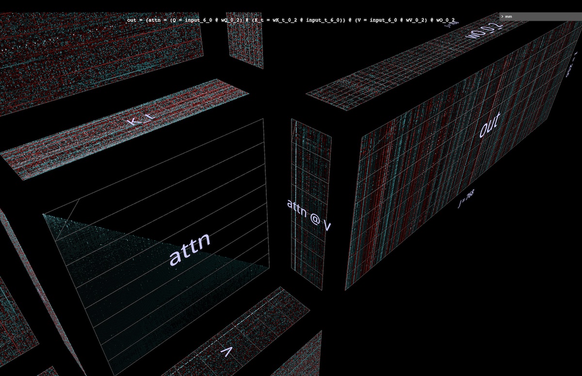
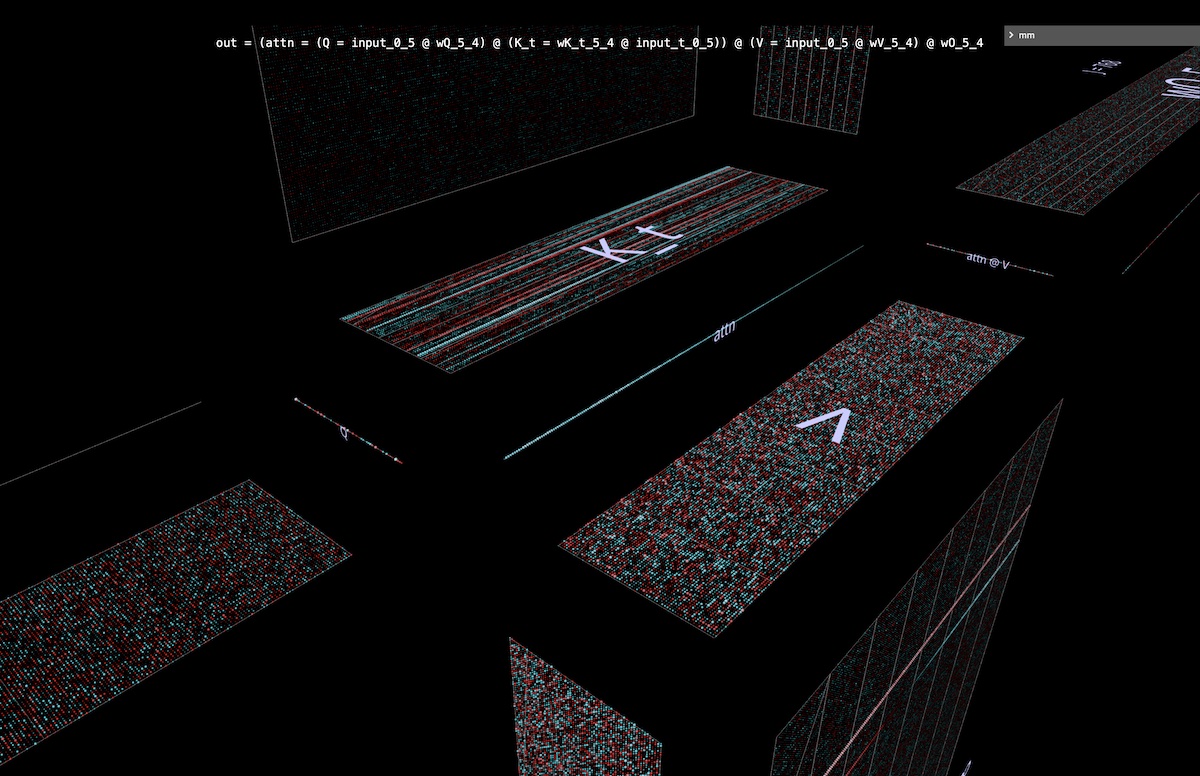
A thumbnail description of what we’re looking at:

• the blades of the windmill are matmuls 1, 2, 3 and 6: the former group are the in-projections from input to Q, K and V; the latter is the out-projection from attn @ V back to the embedding dimension.
• at the hub is the double matmul that first calculates attention scores (convex cube in back), then uses them to produce output tokens from the values vector (concave cube in front). Causality means that the attention scores form a lower triangle.

But I’d encourage exploring this example in the tool itself, rather than relying on the screenshot or the video below to convey just how much signal can be absorbed from it – both about its structure and the actual values flowing through the computation.

4b Computation and Values

Here’s an animation of the attention head computation. Specifically, we’re watching

sdpa(input @ wQ @ K_t) @ V @ wO

(i.e., matmuls 1, 4 , 5 and 6 above, with K_t and V precomputed) being computed as a fused chain of vector-matrix products: each item in the sequence goes all the way from input through attention to output in one step. More on this animation choice in the later section on parallelization, but first let’s look at what the values being computed tell us.

Open in mm

There’s a lot of interesting stuff going on here.

• Before we even get to the attention calculation, it’s quite striking how low-rank Q and K_t are. Zooming in on the Q @ K_t vector-matrix product animation, the situation is even more vivid: a significant number of channels (embedding positions) in both Q and K look more or less constant across the sequence, implying that the useful attention signal is potentially driven by a only smallish subset of the embedding. Understanding and exploiting this phenomenon is one of the threads we’re pulling on as part of the SysML ATOM transformer efficiency project.
• Perhaps most familiar is the strong-but-not-perfect diagonal that emerges in the attention matrix. This is a common pattern, showing up in many of the attention heads of this model (and those of many transformers). It produces localized attention: the value tokens in the small neighborhood immediately preceding an output token’s position largely determine that output token’s content pattern.
• However, the size of this neighborhood and the influence of individual tokens within it vary nontrivially – this can be seen both in the off-diagonal frost in the attention grid, and in the fluctuating patterns of the attn[i] @ V vector-matrix product plane as it descends the attention matrix on its way through the sequence.
• But note that the local neighborhood isn’t the only thing that’s attracting attention: the leftmost column of the attention grid, corresponding to the first token of the sequence, is entirely filled with nonzero (but fluctuating) values, meaning every output token will be influenced to some degree by the first value token.
• Moreover there’s an inexact but discernible oscillation in attention score dominance between the current token neighborhood and the initial token. The period of the oscillation varies, but broadly speaking starts short and then lengthens as one travels down the sequence (evocatively correlated with the quantity of candidate attention tokens for each row, given causality).
• To get a feel for how (attn @ V) is formed, it’s important not to focus on attention in isolation – V is an equal player. Each output item is a weighted average of the entire V vector: at the limit when attention is a perfect diagonal, attn @ V is simply an exact copy of V. Here we see something more textured: visible banding where particular tokens have scored high over a contiguous subsequence of attention rows, superimposed on a matrix visibly similar to to V but with some vertical smearing due to the fat diagonal. (Aside: per the mm reference guide, long-clicking or control-clicking will reveal the actual numeric values of visualized elements.)
• Bear in mind that since we’re in a middle layer (5), the input to this attention head is an intermediate representation, not the original tokenized text. So the patterns seen in the input are themselves thought-provoking – in particular, the strong vertical threads are particular embedding positions whose values are uniformly high magnitude across long stretches of the sequence – sometimes almost the entire thing.
• Interestingly, though, the first vector in the input sequence is distinctive, not only breaking the pattern of these high-magnitude columns but carrying atypical values at almost every position (aside: not visualized here, but this pattern is repeated over multiple sample inputs).

Note: apropos of the last two bullet points, it’s worth reiterating that we’re visualizing computation over a single sample input. In practice I’ve found that each head has a characteristic pattern it will express consistently (though not identically) over a decent collection of samples (and the upcoming attention head browser will provide a collection of samples to play with), but when looking at any visualization that includes activations, it’s important to bear in mind that a full distribution of inputs may influence the ideas and intuitions it provokes it in subtle ways.

Finally, one more pitch to explore the animation directly!

4c Heads are different in interesting ways

Before we move on, here’s one more demonstration of the usefulness of simply poking around a model to see how it works in detail.

This is another attention head from GPT2. It behaves quite differently from layer 5, head 4 above – as one might expect, given that it’s in a very different part of the model. This head is in the very first layer: layer 0, head 2 (open in mm, may take a few seconds to load model weights):

Things to note:

• This head spreads attention very evenly. This has the effect of delivering a relatively unweighted average of V (or rather, the appropriate causal prefix of V) to each row in attn @ V, as can be seen in this animation: as we move down the attention score triangle, the attn[i] @ V vector-matrix product is small fluctuations away from being simply a downscaled, progressively revealed copy of V.
• attn @ V has striking vertical uniformity – in large columnar regions of the embedding, the same value patterns persist over the entire sequence. One can think of these as properties shared by every token.
• Aside: on the one hand one might expect some uniformity in attn @ V given the effect of very evenly spread attention. But each row has been constructed from only a causal subsequence of V rather than the whole thing – why is that not causing more variation, like a progressive morphing as one moves down the sequence? By visual inspection V isn’t uniform along its length, so the answer must lie in some more subtle property of its distribution of values.
• Finally, this head’s output is even more vertically uniform after out-projection
• the strong impression being that the bulk of the information being delivered by this attention head consists of properties which are shared by every token in the sequence. The composition of its output projection weights reinforces this intuition.

Overall, it’s hard to resist the idea that the extremely regular, highly structured information this attention head produces might be obtained by computational means that are a bit… less lavish. Of course this isn’t an unexplored area, but the specificity and richness of signal of the visualized computation has been useful in generating new ideas, and reasoning about existing ones.

4d Revisiting the pitch: invariants for free

Stepping back, it’s worth reiterating that the reason we can visualize nontrivially compound operations like attention heads and have them remain intuitive is that important algebraic properties – like how argument shapes are constrained, or which parallelization axes intersect which operations – don’t require additional thinking: they arise directly from the geometry of the visualized object, rather than being additional rules to keep in mind.

For example, in these attention head visualizations it’s immediately obvious that

• Q and attn @ V are the same length, K and V are the same length, and the lengths of these pairs are independent of each other
• Q and K are the same width, V and attn @ V are the same width, and the widths of these pairs are independent of each other.

These properties are true by construction, as a simple consequence of which parts of the compound structure the constituents inhabit and how they are oriented.

This “properties for free” benefit can be especially useful when exploring variations on a canonical structure – an obvious example being the one-row-high attention matrix in autoregressive token-at-a-time decoding (open in mm):

5 Parallelizing attention

In the animation of head 5, layer 4 above, we visualize 4 of the 6 matmuls in the attention head

as a fused chain of vector-matrix products, confirming the geometric intuition that the entire left-associative chain from input to output is laminar along the shared i axis, and can be parallelized.

5a Example: partitioning along i

To parallelize the computation in practice, we would partition the input into blocks along the i axis. We can visualize this partition in the tool, by specifying that a given axis be partitioned into a particular number of blocks – in these examples we’ll use 8, but there’s nothing special about that number.

Among other things, this visualization makes clear that wQ (for in-projection), K_t and V (for attention) and wO (for out-projection) are needed in their entirety by each parallel computation, since they’re adjacent to the partitioned matrices along those matrices’ unpartitioned dimensions (open in mm):

5b Example: double partitioning

As an example of partitioning along multiple axes, we can visualize some recent work which innovates in this space (Block Parallel Transformer, building on work done in e.g. Flash Attention and its antecedents).

First, BPT partitions along i as described above – and actually extends this horizontal partitioning of the sequence into chunks all the way through the second (FFN) half of the attention layer as well. (We’ll visualize this in a later section.)

To fully attack the context length problem, a second partitioning is then added to MHA – that of the attention calculation itself (i.e., a partition along the j axis of Q @ K_t). The two partitions together divide attention into a grid of blocks (open in mm):

This visualization makes clear

• the effectiveness of this double partitioning as an attack on the context length problem, since we’ve now visibly partitioned every occurrence of sequence length in the attention calculation
• the “reach” of this second partitioning: it’s clear from the geometry that the in-projection computations of K and V can be partitioned along with the core double matmul

Note one subtlety: the visual implication here is that we can also parallelize the subsequent matmul attn @ V along k and sum the partial results split-k style, thus parallelizing the entire double matmul. But the row-wise softmax in sdpa() adds the requirement that each row have all its segments normalized before the corresponding row of attn @ V can be computed, adding an extra row-wise step between the attention calculation and the final matmul.

6 Sizes in an Attention Layer

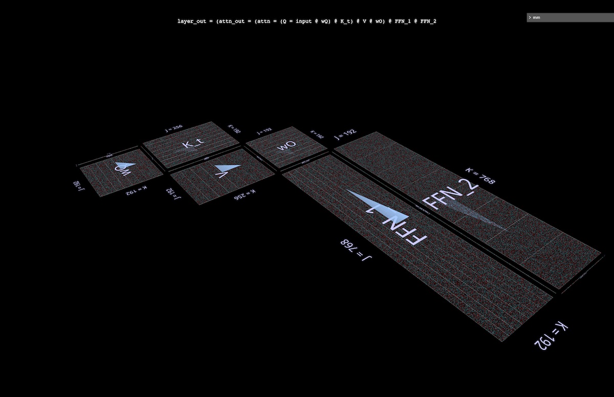
The first (MHA) half of an attention layer is famously computationally demanding because of its quadratic complexity, but the second (FFN) half is demanding in its own right due to the width of its hidden dimension, typically 4 times that of the model’s embedding dimension. Visualizing the biomass of a full attention layer can be useful in building intuition about how the two halves of the layer compare to each other.

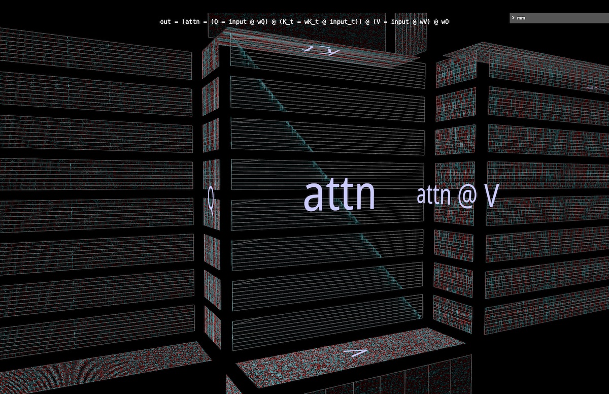
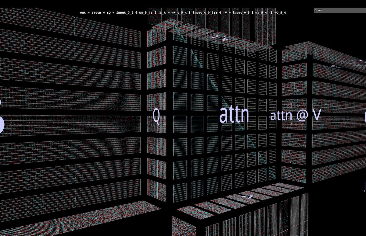
6a Visualizing the full layer

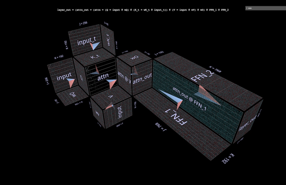
Below is a full attention layer with the first half (MHA) in the background and the second (FFN) in the foreground. As usual, arrows point in the direction of computation.

Notes:

• This visualization doesn’t depict individual attention heads, but instead shows the unsliced Q/K/V weights and projections surrounding a central double matmul. Of course this isn’t a faithful visualization of the full MHA operation – but the goal here is to give a clearer sense of the relative matrix sizes in the two halves of the layer, rather than the relative amounts of computation each half performs. (Also, randomized values are used rather than real weights.)
• The dimensions used here are downsized to keep the browser (relatively) happy, but the proportions are preserved (from NanoGPT’s small config): model embedding dimension = 192 (from 768), FFN embedding dimension = 768 (from 3072), sequence length = 256 (from 1024), although sequence length is not fundamental to the model. (Visually, changes in sequence length would appear as changes in the width of the input blades, and consequently in the size of the attention hub and the height of the downstream vertical planes.)

Open in mm:

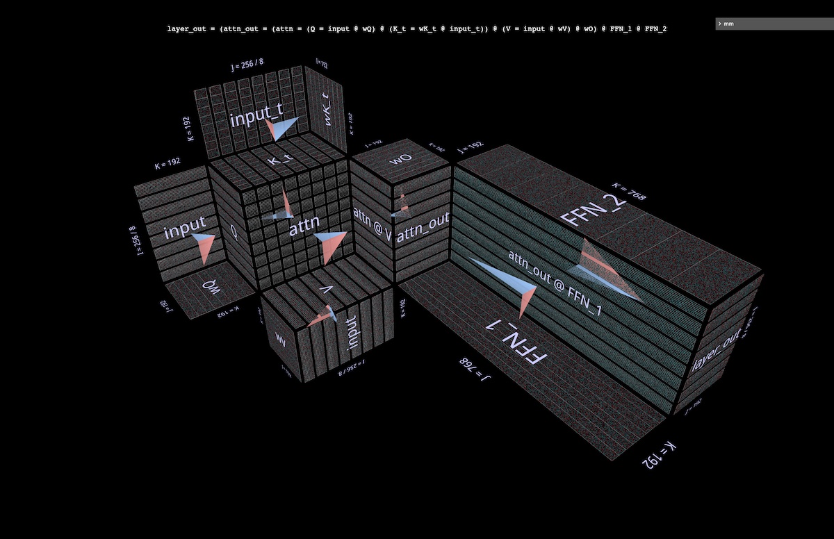
6b Visualizing the BPT partitioned layer

Revisiting Blockwise Parallel Transformer briefly, here we visualize BPT’s parallelization scheme in the context of an entire attention layer (with individual heads elided per above). In particular, note how the partitioning along i (of sequence blocks) extends through both MHA and FFN halves (open in mm):

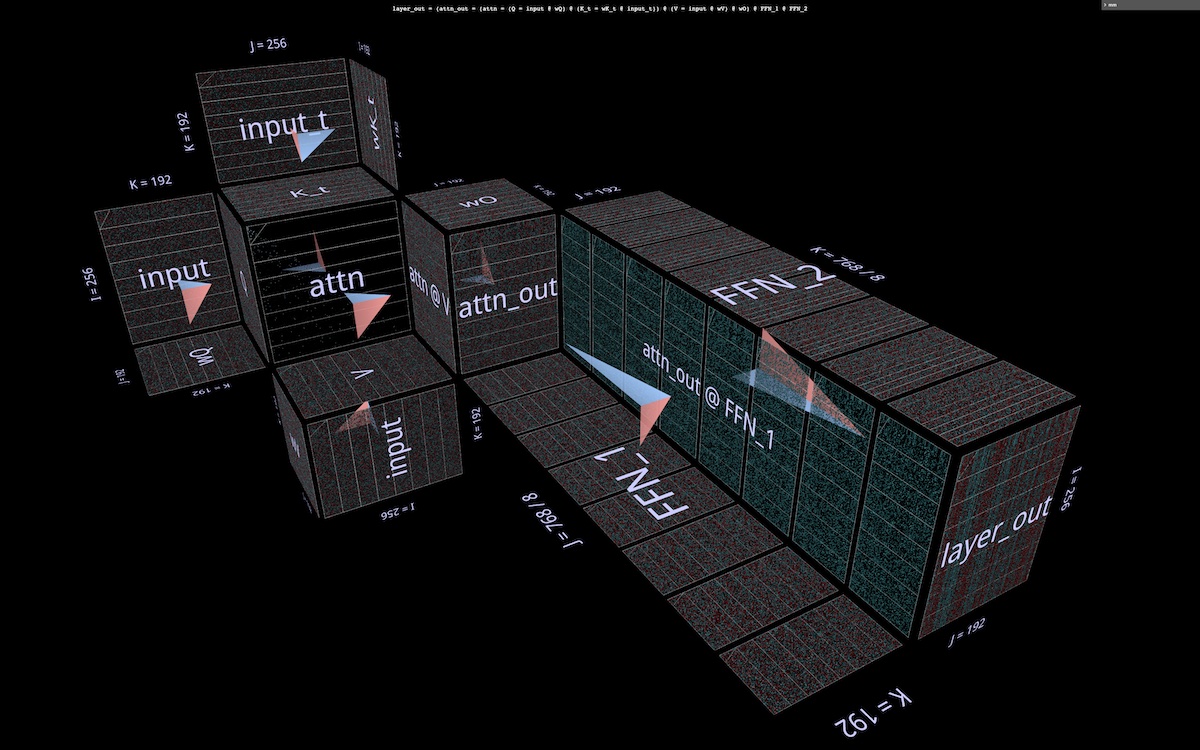
6c Partitioning the FFN

The visualization suggests an additional partitioning, orthogonal to the ones described above – in the FFN half of the attention layer, splitting the double matmul (attn_out @ FFN_1) @ FFN_2, first along j for attn_out @ FFN_1, then along k in the subsequent matmul with FFN_2. This partition slices both layers of FFN weights, reducing the capacity requirements of each participant in the computation at the cost of a final summation of the partial results.

Here’s what this partition looks like applied to an otherwise unpartitioned attention layer (open in mm):

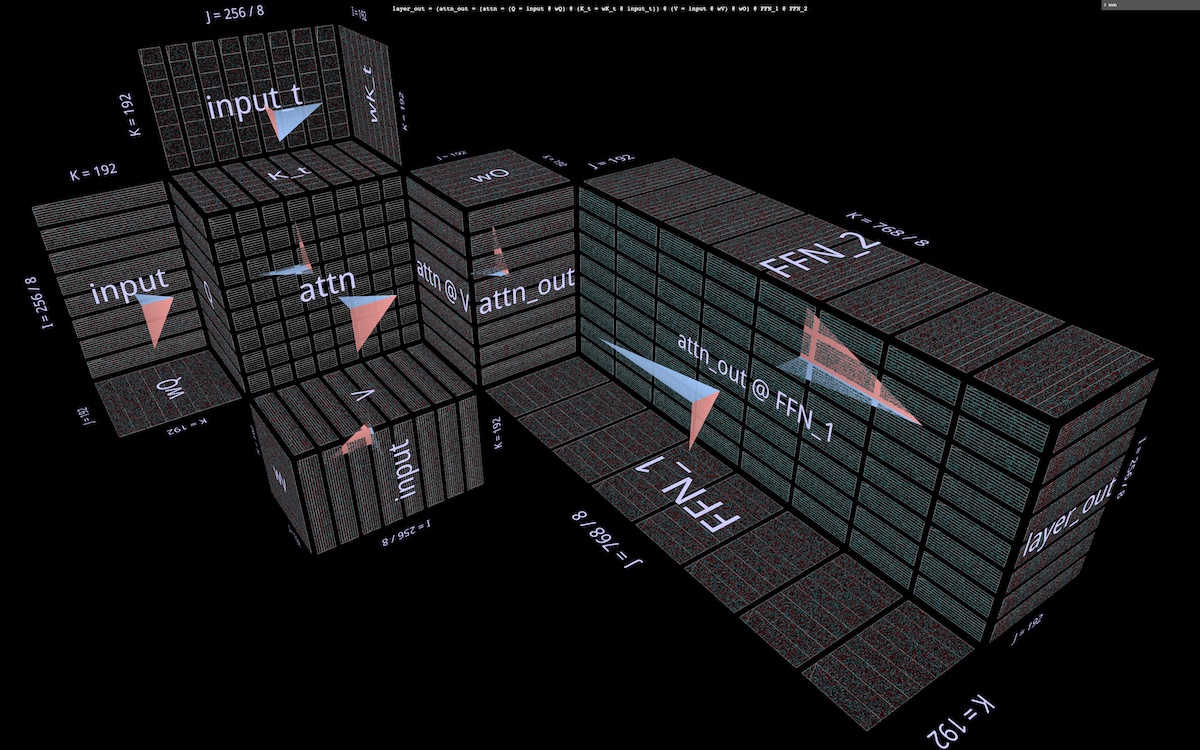
And here it is applied to a layer partitioned a la BPT (open in mm):

6d Visualizing token-at-a-time decoding

During autoregressive token-at-a-time decoding, the query vector consists of a single token. It’s instructive to have a mental picture of what an attention layer looks like in that situation – a single embedding row working its way through an enormous tiled plane of weights.

Aside from the emphasizing the sheer immensity of weights compared to activations, this view is also evocative of the notion that K_t and V function like dynamically generated layers in a 6-layer MLP, although the mux/demux computations of MHA itself (papered over here, per above) make the correspondence inexact (open in mm):

7 LoRA

The recent LoRA paper (LoRA: Low-Rank Adaptation of Large Language Models) describes an efficient finetuning technique based on the idea that weight deltas introduced during finetuning are low-rank. Per the paper, this “allows us to train some dense layers in a neural network indirectly by optimizing rank decomposition matrices of the dense layers’ change during adaptation […], while keeping the pre-trained weights frozen.”

7a The basic idea

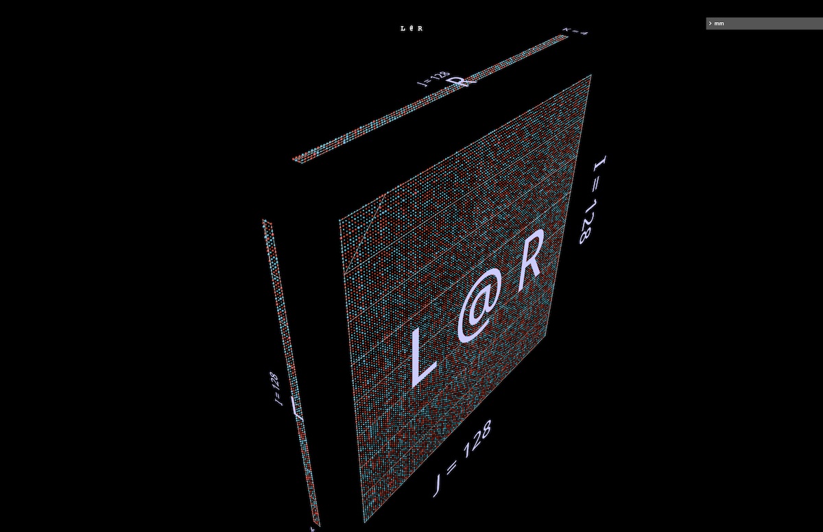
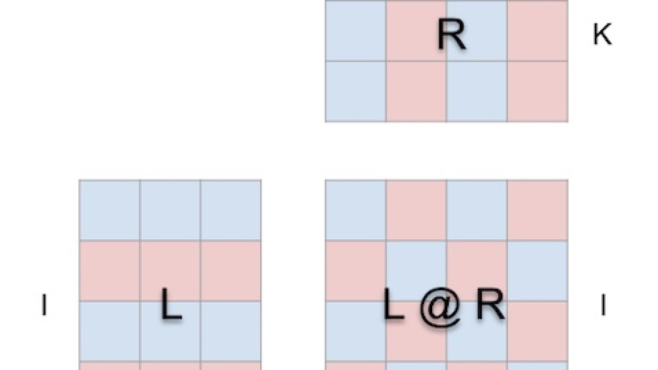
In a nutshell, the key move is to train the factors of a weight matrix rather than the matrix itself: replace an I x J weights tensor with a matmul of an I x K tensor and a K x J tensor, holding K to some small number.

If K is small enough the size win can be huge, but the tradeoff is that lowering it lowers the rank of what the product can express. As a quick illustration of both the size savings and the structuring effect on the result, here’s a matmul of random 128 x 4 left and 4 x 128 right arguments – a.k.a. a rank-4 factorization of a 128 x 128 matrix. Notice the vertical and horizontal patterning in L @ R (open in mm):

7b Applying LoRA to an attention head

The way LoRA applies this factoring move to the fine tuning process is to

• create a low-rank factorization for each weight tensor to be fine-tuned and train the factors, keeping the original weights frozen
• after fine tuning, multiply each pair of low-rank factors to get a matrix in the shape of the original weights tensor, and add it to the original pretrained weights tensor

The following visualization shows an attention head with the weight tensors wQ, wK_t, wV, wO replaced by low rank factorizations wQ_A @ wQ_B, etc. Visually, the factor matrices show up as low fences along the edges of the windmill blades (open in mm – spacebar stops the spin):

8 Wrapup

8a Call for feedback

I’ve found this way of visualizing matmul expressions extremely helpful for building intuition and reasoning about not just matrix multiplication itself, but also many aspects of ML models and their computation, from efficiency to interpretability.

if you try it out and have suggestions or comments, I definitely want to hear, either in the comments here or in the repo.

8b Next steps

• There’s a GPT2 attention head explorer built on top of the tool which I’m currently using to inventory and classify the attention head traits found in that model. (This was the tool I used to find and explore the attention heads in this note.) Once complete I plan to post a note with the inventory.
• As mentioned up top, embedding these visualizations in Python notebooks is dead simple. But session URLs can get… unwieldy, so it will be useful to have Python-side utilities for constructing them from configuration objects, similar to the simple JavaScript helpers used in the reference guide.
• If you’ve got a use case you think might benefit from visualizations like this but it’s not obvious how to use the tool to do it, get in touch! I’m not necessarily looking to expand its core visualization capabilities that much further (right tool for the job, etc.), but e.g. the API for driving it programmatically is pretty basic, there’s plenty that can be done there.

Read More