University of Chicago Pritzker School of Molecular Engineering professor honored for his ‘substantial contributions to the field of theoretical quantum information science’.Read More
Making RL Tractable by Learning More Informative Reward Functions: Example-Based Control, Meta-Learning, and Normalized Maximum Likelihood
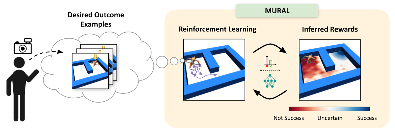
Diagram of MURAL, our method for learning uncertainty-aware rewards for RL. After the user provides a few examples of desired outcomes, MURAL automatically infers a reward function that takes into account these examples and the agent’s uncertainty for each state.
Although reinforcement learning has shown success in domains such as robotics, chip placement and playing video games, it is usually intractable in its most general form. In particular, deciding when and how to visit new states in the hopes of learning more about the environment can be challenging, especially when the reward signal is uninformative. These questions of reward specification and exploration are closely connected — the more directed and “well shaped” a reward function is, the easier the problem of exploration becomes. The answer to the question of how to explore most effectively is likely to be closely informed by the particular choice of how we specify rewards.
For unstructured problem settings such as robotic manipulation and navigation — areas where RL holds substantial promise for enabling better real-world intelligent agents — reward specification is often the key factor preventing us from tackling more difficult tasks. The challenge of effective reward specification is two-fold: we require reward functions that can be specified in the real world without significantly instrumenting the environment, but also effectively guide the agent to solve difficult exploration problems. In our recent work, we address this challenge by designing a reward specification technique that naturally incentivizes exploration and enables agents to explore environments in a directed way.
Saving seaweed with machine learning
Last year, Charlene Xia ’17, SM ’20 found herself at a crossroads. She was finishing up her master’s degree in media arts and sciences from the MIT Media Lab and had just submitted applications to doctoral degree programs. All Xia could do was sit and wait. In the meantime, she narrowed down her career options, regardless of whether she was accepted to any program.
“I had two thoughts: I’m either going to get a PhD to work on a project that protects our planet, or I’m going to start a restaurant,” recalls Xia.
Xia poured over her extensive cookbook collection, researching international cuisines as she anxiously awaited word about her graduate school applications. She even looked into the cost of a food truck permit in the Boston area. Just as she started hatching plans to open a plant-based skewer restaurant, Xia received word that she had been accepted into the mechanical engineering graduate program at MIT.
Shortly after starting her doctoral studies, Xia’s advisor, Professor David Wallace, approached her with an interesting opportunity. MathWorks, a software company known for developing the MATLAB computing platform, had announced a new seed funding program in MIT’s Department of Mechanical Engineering. The program encouraged collaborative research projects focused on the health of the planet.
“I saw this as a super-fun opportunity to combine my passion for food, my technical expertise in ocean engineering, and my interest in sustainably helping our planet,” says Xia.
Wallace knew Xia would be up to the task of taking an interdisciplinary approach to solve an issue related to the health of the planet. “Charlene is a remarkable student with extraordinary talent and deep thoughtfulness. She is pretty much fearless, embracing challenges in almost any domain with the well-founded belief that, with effort, she will become a master,” says Wallace.
Alongside Wallace and Associate Professor Stefanie Mueller, Xia proposed a project to predict and prevent the spread of diseases in aquaculture. The team focused on seaweed farms in particular.
Already popular in East Asian cuisines, seaweed holds tremendous potential as a sustainable food source for the world’s ever-growing population. In addition to its nutritive value, seaweed combats various environmental threats. It helps fight climate change by absorbing excess carbon dioxide in the atmosphere, and can also absorb fertilizer run-off, keeping coasts cleaner.
As with so much of marine life, seaweed is threatened by the very thing it helps mitigate against: climate change. Climate stressors like warm temperatures or minimal sunlight encourage the growth of harmful bacteria such as ice-ice disease. Within days, entire seaweed farms are decimated by unchecked bacterial growth.
To solve this problem, Xia turned to the microbiota present in these seaweed farms as a predictive indicator of any threat to the seaweed or livestock. “Our project is to develop a low-cost device that can detect and prevent diseases before they affect seaweed or livestock by monitoring the microbiome of the environment,” says Xia.
The team pairs old technology with the latest in computing. Using a submersible digital holographic microscope, they take a 2D image. They then use a machine learning system known as a neural network to convert the 2D image into a representation of the microbiome present in the 3D environment.
“Using a machine learning network, you can take a 2D image and reconstruct it almost in real time to get an idea of what the microbiome looks like in a 3D space,” says Xia.
The software can be run in a small Raspberry Pi that could be attached to the holographic microscope. To figure out how to communicate these data back to the research team, Xia drew upon her master’s degree research.
In that work, under the guidance of Professor Allan Adams and Professor Joseph Paradiso in the Media Lab, Xia focused on developing small underwater communication devices that can relay data about the ocean back to researchers. Rather than the usual $4,000, these devices were designed to cost less than $100, helping lower the cost barrier for those interested in uncovering the many mysteries of our oceans. The communication devices can be used to relay data about the ocean environment from the machine learning algorithms.
By combining these low-cost communication devices along with microscopic images and machine learning, Xia hopes to design a low-cost, real-time monitoring system that can be scaled to cover entire seaweed farms.
“It’s almost like having the ‘internet of things’ underwater,” adds Xia. “I’m developing this whole underwater camera system alongside the wireless communication I developed that can give me the data while I’m sitting on dry land.”
Armed with these data about the microbiome, Xia and her team can detect whether or not a disease is about to strike and jeopardize seaweed or livestock before it is too late.
While Xia still daydreams about opening a restaurant, she hopes the seaweed project will prompt people to rethink how they consider food production in general.
“We should think about farming and food production in terms of the entire ecosystem,” she says. “My meta-goal for this project would be to get people to think about food production in a more holistic and natural way.”
Alexa & Friends features Pradeep Natarajan, Alexa AI principal applied scientist
Natarajan discusses his work in the field of computer vision, machine learning, and multimedia processing.Read More
Practical Differentially Private Clustering
Posted by Alisa Chang, Software Engineer, Google Cloud and Pritish Kamath, Research Scientist, Google Research
Over the last several years, progress has been made on privacy-safe approaches for handling sensitive data, for example, while discovering insights into human mobility and through use of federated analytics such as RAPPOR. In 2019, we released an open source library to enable developers and organizations to use techniques that provide differential privacy, a strong and widely accepted mathematical notion of privacy. Differentially-private data analysis is a principled approach that enables organizations to learn and release insights from the bulk of their data while simultaneously providing a mathematical guarantee that those results do not allow any individual user’s data to be distinguished or re-identified.
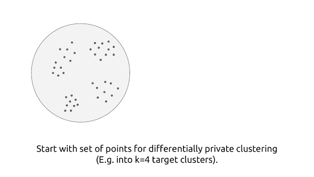
In this post, we consider the following basic problem: Given a database containing several attributes about users, how can one create meaningful user groups and understand their characteristics? Importantly, if the database at hand contains sensitive user attributes, how can one reveal these group characteristics without compromising the privacy of individual users?
Such a task falls under the broad umbrella of clustering, a fundamental building block in unsupervised machine learning. A clustering method partitions the data points into groups and provides a way to assign any new data point to a group with which it is most similar. The k-means clustering algorithm has been one such influential clustering method. However, when working with sensitive datasets, it can potentially reveal significant information about individual data points, putting the privacy of the corresponding user at risk.
Today, we announce the addition of a new differentially private clustering algorithm to our differential privacy library, which is based on privately generating new representative data points. We evaluate its performance on multiple datasets and compare to existing baselines, finding competitive or better performance.
K-means Clustering
Given a set of data points, the goal of k-means clustering is to identify (at most) k points, called cluster centers, so as to minimize the loss given by the sum of squared distances of the data points from their closest cluster center. This partitions the set of data points into k groups. Moreover, any new data point can be assigned to a group based on its closest cluster center. However, releasing the set of cluster centers has the potential to leak information about particular users — for example, consider a scenario where a particular data point is significantly far from the rest of the points, so the standard k-means clustering algorithm returns a cluster center at this single point, thereby revealing sensitive information about this single point. To address this, we design a new algorithm for clustering with the k-means objective within the framework of differential privacy.
A Differentially Private Algorithm
In “Locally Private k-Means in One Round”, published at ICML 2021, we presented a differentially private algorithm for clustering data points. That algorithm had the advantage of being private in the local model, where the user’s privacy is protected even from the central server performing the clustering. However, any such approach necessarily incurs a significantly larger loss than approaches using models of privacy that require trusting a central server.1
Here, we present a similarly inspired clustering algorithm that works in the central model of differential privacy, where the central server is trusted to have complete access to the raw data, and the goal is to compute differentially private cluster centers, which do not leak information about individual data points. The central model is the standard model for differential privacy, and algorithms in the central model can be more easily substituted in place of their non-private counterparts since they do not require changes to the data collection process. The algorithm proceeds by first generating, in a differentially private manner, a core-set that consists of weighted points that “represent” the data points well. This is followed by executing any (non-private) clustering algorithm (e.g., k-means++) on this privately generated core-set.
At a high level, the algorithm generates the private core-set by first using random-projection–based locality-sensitive hashing (LSH) in a recursive manner2 to partition the points into “buckets” of similar points, and then replacing each bucket by a single weighted point that is the average of the points in the bucket, with a weight equal to the number of points in the same bucket. As described so far, though, this algorithm is not private. We make it private by performing each operation in a private manner by adding noise to both the counts and averages of points within a bucket.
This algorithm satisfies differential privacy because each point’s contributions to the bucket counts and the bucket averages are masked by the added noise, so the behavior of the algorithm does not reveal information about any individual point. There is a tradeoff with this approach: if the number of points in the buckets is too large, then individual points will not be well-represented by points in the core-set, whereas if the number of points in a bucket is too small, then the added noise (to the counts and averages) will become significant in comparison to the actual values, leading to poor quality of the core-set. This trade-off is realized with user-provided parameters in the algorithm that control the number of points that can be in a bucket.
|
| Visual illustration of the algorithm. |
Experimental Evaluation
We evaluated the algorithm on a few benchmark datasets, comparing its performance to that of the (non-private) k-means++ algorithm, as well as a few other algorithms with available implementations, namely diffprivlib and dp-clustering-icml17. We use the following benchmark datasets: (i) a synthetic dataset consisting of 100,000 data points in 100 dimensions sampled from a mixture of 64 Gaussians; (ii) neural representations for the MNIST dataset on handwritten digits obtained by training a LeNet model; (iii) the UC Irvine dataset on Letter Recognition; and (iv) the UC Irvine dataset on Gas Turbine CO and NOx Emissions.3
We analyze the normalized k-means loss (mean squared distance from data points to the nearest center) while varying the number of target centers (k) for these benchmark datasets.4 The described algorithm achieves a lower loss than the other private algorithms in three out of the four datasets we consider.
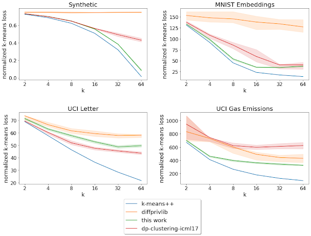 |
| Normalized loss for varying k = number of target clusters (lower is better). The solid curves denote the mean over the 20 runs, and the shaded region denotes the 25-75th percentile range. |
Moreover, for datasets with specified ground-truth labels (i.e., known groupings), we analyze the cluster label accuracy, which is the accuracy of the labeling obtained by assigning the most frequent ground-truth label in each cluster found by the clustering algorithm to all points in that cluster. Here, the described algorithm performs better than other private algorithms for all the datasets with pre-specified ground-truth labels that we consider.
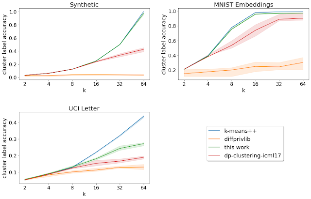 |
| Cluster label accuracy for varying k = number of target clusters (higher is better). The solid curves denote the mean over the 20 runs, and the shaded region denotes the 25-75th percentile range. |
Limitations and Future Directions
There are a couple of limitations to consider when using this or any other library for private clustering.
- It is important to separately account for the privacy loss in any preprocessing (e.g., centering the data points or rescaling the different coordinates) done before using the private clustering algorithm. So, we hope to provide support for differentially private versions of commonly used preprocessing methods in the future and investigate changes so that the algorithm performs better with data that isn’t necessarily preprocessed.
- The algorithm described requires a user-provided radius, such that all data points lie within a sphere of that radius. This is used to determine the amount of noise that is added to the bucket averages. Note that this differs from diffprivlib and dp-clustering-icml17 which take in different notions of bounds of the dataset (e.g., a minimum and maximum of each coordinate). For the sake of our experimental evaluation, we calculated the relevant bounds non-privately for each dataset. However, when running the algorithms in practice, these bounds should generally be privately computed or provided without knowledge of the dataset (e.g., using the underlying range of the data). Although, note that in case of the algorithm described, the provided radius need not be exactly correct; any data points outside of the provided radius are replaced with the closest points that are within the sphere of that radius.
Conclusion
This work proposes a new algorithm for computing representative points (cluster centers) within the framework of differential privacy. With the rise in the amount of datasets collected around the world, we hope that our open source tool will help organizations obtain and share meaningful insights about their datasets, with the mathematical assurance of differential privacy.
Acknowledgements
We thank Christoph Dibak, Badih Ghazi, Miguel Guevara, Sasha Kulankhina, Ravi Kumar, Pasin Manurangsi, Jane Shapiro, Daniel Simmons-Marengo, Yurii Sushko, and Mirac Vuslat Basaran for their help.
1As shown by Uri Stemmer in Locally private k-means clustering (SODA 2020). ↩
2This is similar to work on LSH Forest, used in the context of similarity-search queries. ↩
3Datasets (iii) and (iv) were centered to have mean zero before evaluating the algorithms. ↩
4Evaluation done for fixed privacy parameters ε = 1.0 and δ = 1e-6. Note that dp-clustering-icml17 works in the pure differential privacy model (namely, with δ = 0); k-means++, of course, has no privacy parameters. ↩

Bits into atoms, atoms into bits
A third digital revolution is coming, and Neil Gershenfeld is at the forefront.Read More
New Library Releases in PyTorch 1.10, including TorchX, TorchAudio, TorchVision
Today, we are announcing a number of new features and improvements to PyTorch libraries, alongside the PyTorch 1.10 release. Some highlights include:
Some highlights include:
- TorchX – a new SDK for quickly building and deploying ML applications from research & development to production.
- TorchAudio – Added text-to-speech pipeline, self-supervised model support, multi-channel support and MVDR beamforming module, RNN transducer (RNNT) loss function, and batch and filterbank support to
lfilterfunction. See the TorchAudio release notes here. - TorchVision – Added new RegNet and EfficientNet models, FX based feature extraction added to utilities, two new Automatic Augmentation techniques: Rand Augment and Trivial Augment, and updated training recipes. See the TorchVision release notes here.
Introducing TorchX
TorchX is a new SDK for quickly building and deploying ML applications from research & development to production. It offers various builtin components that encode MLOps best practices and make advanced features like distributed training and hyperparameter optimization accessible to all.
Users can get started with TorchX 0.1 with no added setup cost since it supports popular ML schedulers and pipeline orchestrators that are already widely adopted and deployed in production. No two production environments are the same. To comply with various use cases, TorchX’s core APIs allow tons of customization at well-defined extension points so that even the most unique applications can be serviced without customizing the whole vertical stack.
Read the documentation for more details and try out this feature using this quickstart tutorial.
TorchAudio 0.10
[Beta] Text-to-speech pipeline
TorchAudio now adds the Tacotron2 model and pretrained weights. It is now possible to build a text-to-speech pipeline with existing vocoder implementations like WaveRNN and Griffin-Lim. Building a TTS pipeline requires matching data processing and pretrained weights, which are often non-trivial to users. So TorchAudio introduces a bundle API so that constructing pipelines for specific pretrained weights is easy. The following example illustrates this.
>>> import torchaudio
>>>
>>> bundle = torchaudio.pipelines.TACOTRON2_WAVERNN_CHAR_LJSPEECH
>>>
>>> # Build text processor, Tacotron2 and vocoder (WaveRNN) model
>>> processor = bundle.get_text_processor()
>>> tacotron2 = bundle.get_tacotron2()
Downloading:
100%|███████████████████████████████| 107M/107M [00:01<00:00, 87.9MB/s]
>>> vocoder = bundle.get_vocoder()
Downloading:
100%|███████████████████████████████| 16.7M/16.7M [00:00<00:00, 78.1MB/s]
>>>
>>> text = "Hello World!"
>>>
>>> # Encode text
>>> input, lengths = processor(text)
>>>
>>> # Generate (mel-scale) spectrogram
>>> specgram, lengths, _ = tacotron2.infer(input, lengths)
>>>
>>> # Convert spectrogram to waveform
>>> waveforms, lengths = vocoder(specgram, lengths)
>>>
>>> # Save audio
>>> torchaudio.save('hello-world.wav', waveforms, vocoder.sample_rate)
For the details of this API please refer to the documentation. You can also try this from the tutorial.
(Beta) Self-Supervised Model Support
TorchAudio added HuBERT model architecture and pre-trained weight support for wav2vec 2.0 and HuBERT. HuBERT and wav2vec 2.0 are novel ways for audio representation learning and they yield high accuracy when fine-tuned on downstream tasks. These models can serve as baseline in future research, therefore, TorchAudio is providing a simple way to run the model. Similar to the TTS pipeline, the pretrained weights and associated information, such as expected sample rates and output class labels (for fine-tuned weights) are put together as a bundle, so that they can be used to build pipelines. The following example illustrates this.
>>> import torchaudio
>>>
>>> bundle = torchaudio.pipelines.HUBERT_ASR_LARGE
>>>
>>> # Build the model and load pretrained weight.
>>> model = bundle.get_model()
Downloading:
100%|███████████████████████████████| 1.18G/1.18G [00:17<00:00, 73.8MB/s]
>>> # Check the corresponding labels of the output.
>>> labels = bundle.get_labels()
>>> print(labels)
('<s>', '<pad>', '</s>', '<unk>', '|', 'E', 'T', 'A', 'O', 'N', 'I', 'H', 'S', 'R', 'D', 'L', 'U', 'M', 'W', 'C', 'F', 'G', 'Y', 'P', 'B', 'V', 'K', "'", 'X', 'J', 'Q', 'Z')
>>>
>>> # Infer the label probability distribution
>>> waveform, sample_rate = torchaudio.load(hello-world.wav')
>>>
>>> emissions, _ = model(waveform)
>>>
>>> # Pass emission to (hypothetical) decoder
>>> transcripts = ctc_decode(emissions, labels)
>>> print(transcripts[0])
HELLO WORLD
Please refer to the documentation for more details and try out this feature using this tutorial.
(Beta) Multi-channel support and MVDR beamforming
Far-field speech recognition is a more challenging task compared to near-field recognition. Multi-channel methods such as beamforming help reduce the noises and enhance the target speech.
TorchAudio now adds support for differentiable Minimum Variance Distortionless Response (MVDR) beamforming on multi-channel audio using Time-Frequency masks. Researchers can easily assemble it with any multi-channel ASR pipeline. There are three solutions (ref_channel, stv_evd, stv_power) and it supports single-channel and multi-channel (perform average in the method) masks. It provides an online option that recursively updates the parameters for streaming audio. We also provide a tutorial on how to apply MVDR beamforming to the multi-channel audio in the example directory.
>>> from torchaudio.transforms import MVDR, Spectrogram, InverseSpectrogram
>>>
>>> # Load the multi-channel noisy audio
>>> waveform_mix, sr = torchaudio.load('mix.wav')
>>> # Initialize the stft and istft modules
>>> stft = Spectrogram(n_fft=1024, hop_length=256, return_complex=True, power=None)
>>> istft = InverseSpectrogram(n_fft=1024, hop_length=256)
>>> # Get the noisy spectrogram
>>> specgram_mix = stft(waveform_mix)
>>> # Get the Time-Frequency mask via machine learning models
>>> mask = model(waveform)
>>> # Initialize the MVDR module
>>> mvdr = MVDR(ref_channel=0, solution=”ref_channel”, multi_mask=False)
>>> # Apply MVDR beamforming
>>> specgram_enhanced = mvdr(specgram_mix, mask)
>>> # Get the enhanced waveform via iSTFT
>>> waveform_enhanced = istft(specgram_enhanced, length=waveform.shape[-1])
Please refer to the documentation for more details and try out this feature using the MVDR tutorial.
(Beta) RNN Transducer Loss
The RNN transducer (RNNT) loss is part of the RNN transducer pipeline, which is a popular architecture for speech recognition tasks. Recently it has gotten attention for being used in a streaming setting, and has also achieved state-of-the-art WER for the LibriSpeech benchmark.
TorchAudio’s loss function supports float16 and float32 logits, has autograd and torchscript support, and can be run on both CPU and GPU, which has a custom CUDA kernel implementation for improved performance. The implementation is consistent with the original loss function in Sequence Transduction with Recurrent Neural Networks, but relies on code from Alignment Restricted Streaming Recurrent Neural Network Transducer. Special thanks to Jay Mahadeokar and Ching-Feng Yeh for their code contributions and guidance.
Please refer to the documentation for more details.
(Beta) Batch support and filter bank support
torchaudio.functional.lfilter now supports batch processing and multiple filters.
(Prototype) Emformer Module
Automatic speech recognition (ASR) research and productization have increasingly focused on on-device applications. Towards supporting such efforts, TorchAudio now includes Emformer, a memory-efficient transformer architecture that has achieved state-of-the-art results on LibriSpeech in low-latency streaming scenarios, as a prototype feature.
Please refer to the documentation for more details.
GPU Build
GPU builds that support custom CUDA kernels in TorchAudio, like the one being used for RNN transducer loss, have been added. Following this change, TorchAudio’s binary distribution now includes CPU-only versions and CUDA-enabled versions. To use CUDA-enabled binaries, PyTorch also needs to be compatible with CUDA.
TorchVision 0.11
(Stable) New Models
RegNet and EfficientNet are two popular architectures that can be scaled to different computational budgets. In this release we include 22 pre-trained weights for their classification variants. The models were trained on ImageNet and the accuracies of the pre-trained models obtained on ImageNet val can be found below (see #4403, #4530 and #4293 for more details).
The models can be used as follows:
import torch
from torchvision import models

x = torch.rand(1, 3, 224, 224)

regnet = models.regnet_y_400mf(pretrained=True)
regnet.eval()
predictions = regnet(x)

efficientnet = models.efficientnet_b0(pretrained=True)
efficientnet.eval()
predictions = efficientnet(x)
See the full list of new models on the torchvision.models documentation page.
We would like to thank Ross Wightman and Luke Melas-Kyriazi for contributing the weights of the EfficientNet variants.
(Beta) FX-based Feature Extraction
A new Feature Extraction method has been added to our utilities. It uses torch.fx and enables us to retrieve the outputs of intermediate layers of a network which is useful for feature extraction and visualization.
Here is an example of how to use the new utility:
import torch
from torchvision.models import resnet50
from torchvision.models.feature_extraction import create_feature_extractor


x = torch.rand(1, 3, 224, 224)

model = resnet50()

return_nodes = {
"layer4.2.relu_2": "layer4"
}
model2 = create_feature_extractor(model, return_nodes=return_nodes)
intermediate_outputs = model2(x)

print(intermediate_outputs['layer4'].shape)
We would like to thank Alexander Soare for developing this utility.
(Stable) New Data Augmentations
Two new Automatic Augmentation techniques were added: RandAugment and Trivial Augment. They apply a series of transformations on the original data to enhance them and to boost the performance of the models. The new techniques build on top of the previously added AutoAugment and focus on simplifying the approach, reducing the search space for the optimal policy and improving the performance gain in terms of accuracy. These techniques enable users to reproduce recipes to achieve state-of-the-art performance on the offered models. Additionally, it enables users to apply these techniques in order to do transfer learning and achieve optimal accuracy on new datasets.
Both methods can be used as drop-in replacement of the AutoAugment technique as seen below:
from torchvision import transforms

t = transforms.RandAugment()
# t = transforms.TrivialAugmentWide()
transformed = t(image)

transform = transforms.Compose([
transforms.Resize(256),
transforms.RandAugment(), # transforms.TrivialAugmentWide()
transforms.ToTensor()])
Read the automatic augmentation transforms for more details.
We would like to thank Samuel G. Müller for contributing to Trivial Augment and for his help on refactoring the AA package.
Updated Training Recipes
We have updated our training reference scripts to add support for Exponential Moving Average, Label Smoothing, Learning-Rate Warmup, Mixup, Cutmix and other SOTA primitives. The above enabled us to improve the classification Acc@1 of some pre-trained models by over 4 points. A major update of the existing pre-trained weights is expected in the next release.
Thanks for reading. If you’re interested in these updates and want to join the PyTorch community, we encourage you to join the discussion forums and open GitHub issues. To get the latest news from PyTorch, follow us on Twitter, Medium, YouTube and LinkedIn.
Cheers!
Team PyTorch
PyTorch 1.10 Release, including CUDA Graphs APIs, Frontend and Compiler Improvements
We are excited to announce the release of PyTorch 1.10. This release is composed of over 3,400 commits since 1.9, made by 426 contributors. We want to sincerely thank our community for continuously improving PyTorch.
PyTorch 1.10 updates are focused on improving training and performance of PyTorch, and developer usability. The full release notes are available here. Highlights include:
- CUDA Graphs APIs are integrated to reduce CPU overheads for CUDA workloads.
- Several frontend APIs such as FX, torch.special, and nn.Module Parametrization, have moved from beta to stable.
- Support for automatic fusion in JIT Compiler expands to CPUs in addition to GPUs.
- Android NNAPI support is now available in beta.
Along with 1.10, we are also releasing major updates to the PyTorch libraries, which you can read about in this blog post.
Frontend APIs
(Stable) Python code transformations with FX
FX provides a Pythonic platform for transforming and lowering PyTorch programs. It is a toolkit for pass writers to facilitate Python-to-Python transformation of functions and nn.Module instances. This toolkit aims to support a subset of Python language semantics—rather than the whole Python language—to facilitate ease of implementation of transforms. With 1.10, FX is moving to stable.
You can learn more about FX in the official documentation and GitHub examples of program transformations implemented using torch.fx.
(Stable) torch.special
A torch.special module, analogous to SciPy’s special module, is now available in stable. The module has 30 operations, including gamma, Bessel, and (Gauss) error functions.
Refer to this documentation for more details.
(Stable) nn.Module Parametrization
nn.Module parametrizaton, a feature that allows users to parametrize any parameter or buffer of an nn.Module without modifying the nn.Module itself, is available in stable. This release adds weight normalization (weight_norm), orthogonal parametrization (matrix constraints and part of pruning) and more flexibility when creating your own parametrization.
Refer to this tutorial and the general documentation for more details.
(Beta) CUDA Graphs APIs Integration
PyTorch now integrates CUDA Graphs APIs to reduce CPU overheads for CUDA workloads.
CUDA Graphs greatly reduce the CPU overhead for CPU-bound cuda workloads and thus improve performance by increasing GPU utilization. For distributed workloads, CUDA Graphs also reduce jitter, and since parallel workloads have to wait for the slowest worker, reducing jitter improves overall parallel efficiency.
Integration allows seamless interop between the parts of the network captured by cuda graphs, and parts of the network that cannot be captured due to graph limitations.
Read the note for more details and examples, and refer to the general documentation for additional information.
[Beta] Conjugate View
PyTorch’s conjugation for complex tensors (torch.conj()) is now a constant time operation, and returns a view of the input tensor with a conjugate bit set as can be seen by calling torch.is_conj() . This has already been leveraged in various other PyTorch operations like matrix multiplication, dot product etc., to fuse conjugation with the operation leading to significant performance gain and memory savings on both CPU and CUDA.
Distributed Training
Distributed Training Releases Now in Stable
In 1.10, there are a number of features that are moving from beta to stable in the distributed package:
- (Stable) Remote Module: This feature allows users to operate a module on a remote worker like using a local module, where the RPCs are transparent to the user. Refer to this documentation for more details.
- (Stable) DDP Communication Hook: This feature allows users to override how DDP synchronizes gradients across processes. Refer to this documentation for more details.
- (Stable) ZeroRedundancyOptimizer: This feature can be used in conjunction with DistributedDataParallel to reduce the size of per-process optimizer states. With this stable release, it now can handle uneven inputs to different data-parallel workers. Check out this tutorial. We also improved the parameter partition algorithm to better balance memory and computation overhead across processes. Refer to this documentation and this tutorial to learn more.
Performance Optimization and Tooling
[Beta] Profile-directed typing in TorchScript
TorchScript has a hard requirement for source code to have type annotations in order for compilation to be successful. For a long time, it was only possible to add missing or incorrect type annotations through trial and error (i.e., by fixing the type-checking errors generated by torch.jit.script one by one), which was inefficient and time consuming.
Now, we have enabled profile directed typing for torch.jit.script by leveraging existing tools like MonkeyType, which makes the process much easier, faster, and more efficient. For more details, refer to the documentation.
(Beta) CPU Fusion
In PyTorch 1.10, we’ve added an LLVM-based JIT compiler for CPUs that can fuse together sequences of torch library calls to improve performance. While we’ve had this capability for some time on GPUs, this release is the first time we’ve brought compilation to the CPU.
You can check out a few performance results for yourself in this Colab notebook.
(Beta) PyTorch Profiler
The objective of PyTorch Profiler is to target the execution steps that are the most costly in time and/or memory, and visualize the workload distribution between GPUs and CPUs. PyTorch 1.10 includes the following key features:
- Enhanced Memory View: This helps you understand your memory usage better. This tool will help you avoid Out of Memory errors by showing active memory allocations at various points of your program run.
- Enhanced Automated Recommendations: This helps provide automated performance recommendations to help optimize your model. The tools recommend changes to batch size, TensorCore, memory reduction technologies, etc.
- Enhanced Kernel View: Additional columns show grid and block sizes as well as shared memory usage and registers per thread.
- Distributed Training: Gloo is now supported for distributed training jobs.
- Correlate Operators in the Forward & Backward Pass: This helps map the operators found in the forward pass to the backward pass, and vice versa, in a trace view.
- TensorCore: This tool shows the Tensor Core (TC) usage and provides recommendations for data scientists and framework developers.
- NVTX: Support for NVTX markers was ported from the legacy autograd profiler.
- Support for profiling on mobile devices: The PyTorch profiler now has better integration with TorchScript and mobile backends, enabling trace collection for mobile workloads.
Refer to this documentation for details. Check out this tutorial to learn how to get started with this feature.
PyTorch Mobile
(Beta) Android NNAPI Support in Beta
Last year we released prototype support for Android’s Neural Networks API (NNAPI). NNAPI allows Android apps to run computationally intensive neural networks on the most powerful and efficient parts of the chips that power mobile phones, including GPUs (Graphics Processing Units) and NPUs (specialized Neural Processing Units).
Since the prototype we’ve added more op coverage, added support for load-time flexible shapes and ability to run the model on the host for testing. Try out this feature using the tutorial.
Additionally, Transfer Learning steps have been added to Object Detection examples. Check out this GitHub page to learn more. Please provide your feedback or ask questions on the forum. You can also check out this presentation to get an overview.
Thanks for reading. If you’re interested in these updates and want to join the PyTorch community, we encourage you to join the discussion forums and open GitHub issues. To get the latest news from PyTorch, follow us on Twitter, Medium, YouTube, and LinkedIn.
Cheers!
Team PyTorch

Predicting Spreadsheet Formulas from Semi-structured Contexts
Posted by Rishabh Singh, Research Scientist and Max Lin, Software Engineer, Google Research
Hundreds of millions of people use spreadsheets, and formulas in those spreadsheets allow users to perform sophisticated analyses and transformations on their data. Although formula languages are simpler than general-purpose programming languages, writing these formulas can still be tedious and error-prone, especially for end-users. We’ve previously developed tools to understand patterns in spreadsheet data to automatically fill missing values in a column, but they were not built to support the process of writing formulas.
In “SpreadsheetCoder: Formula Prediction from Semi-structured Context“, published at ICML 2021, we describe a new model that learns to automatically generate formulas based on the rich context around a target cell. When a user starts writing a formula with the “=” sign in a target cell, the system generates possible relevant formulas for that cell by learning patterns of formulas in historical spreadsheets. The model uses the data present in neighboring rows and columns of the target cell as well as the header row as context. It does this by first embedding the contextual structure of a spreadsheet table, consisting of neighboring and header cells, and then generates the desired spreadsheet formula using this contextual embedding. The formula is generated as two components: 1) the sequence of operators (e.g., SUM, IF, etc.), and 2) the corresponding ranges on which the operators are applied (e.g., “A2:A10”). The feature based on this model is now generally available to Google Sheets users.
|
| Given the user’s intent to enter a formula in cells B7, C7, and D7, the system automatically infers the most likely formula the user might want to write in those cells. |
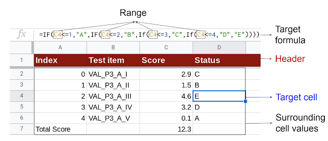 |
| Given the target cell (D4), the model uses the header and surrounding cell values as context to generate the target formula consisting of the corresponding sequence of operators and range. |
Model Architecture
The model uses an encoder-decoder architecture that allows the flexibility to embed multiple types of contextual information (such as that contained in neighboring rows, columns, headers, etc.) in the encoder, which the decoder can use to generate desired formulas. To compute the embedding of the tabular context, it first uses a BERT-based architecture to encode several rows above and below the target cell (together with the header row). The content in each cell includes its data type (such as numeric, string, etc.) and its value, and the cell contents present in the same row are concatenated together into a token sequence to be embedded using the BERT encoder. Similarly, it encodes several columns to the left and to the right of the target cell. Finally, it performs a row-wise and column-wise convolution on the two BERT encoders to compute an aggregated representation of the context.
The decoder uses a long short-term memory (LSTM) architecture to generate the desired target formula as a sequence of tokens by first predicting a formula-sketch (consisting of formula operators without ranges) and then generating the corresponding ranges using cell addresses relative to the target cell. It additionally leverages an attention mechanism to compute attention vectors over the header and cell data, which are concatenated to the LSTM output layer before making the predictions.
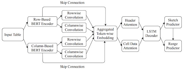 |
| The overall architecture of the formula prediction model. |
In addition to the data present in neighboring rows and columns, the model also leverages additional information from the high-level sheet structure, such as headers. Using TPUs for model predictions, we ensure low latency on generating formula suggestions and are able to handle more requests on fewer machines.
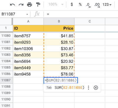 |
| Leveraging the high-level spreadsheet structure, the model can learn ranges that span thousands of rows. |
Results
In the paper, we trained the model on a corpus of spreadsheets created by and shared with Googlers. We split 46k Google Sheets with formulas into 42k for training, 2.3k for validation, and 1.7k for testing. The model achieves a 42.5% top-1 full-formula accuracy, and 57.4% top-1 formula-sketch accuracy, both of which we find high enough to be practically useful in our initial user studies. We perform an ablation study, in which we test several simplifications of the model by removing different components, and find that having row- and column-based context embedding as well as header information is important for models to perform well.
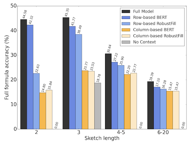 |
| The performance of different ablations of our model with increasing lengths of the target formula. |
Conclusion
Our model illustrates the benefits of learning to represent the two-dimensional relational structure of the spreadsheet tables together with high-level structural information, such as table headers, to facilitate formula predictions. There are several exciting research directions, both in terms of designing new model architectures to incorporate more tabular structure as well as extending the model to support more applications such as bug detection and automated chart creation in spreadsheets. We are also looking forward to seeing how users use this feature and learning from feedback for future improvements.
Acknowledgements
We gratefully acknowledge the key contributions of the other team members, including Alexander Burmistrov, Xinyun Chen, Hanjun Dai, Prashant Khurana, Petros Maniatis, Rahul Srinivasan, Charles Sutton, Amanuel Taddesse, Peilun Zhang, and Denny Zhou.