Introducing the 2021 Facebook India Tech Scholars

Earlier this year, Facebook India launched the Facebook India Tech Scholars (FITS) program to provide a research and mentorship platform to law students who are keen to engage on contemporary questions of technology, law, and policy. Shardul Amarchand Mangaldas & Co. (SAM), India’s foremost full-service law firm, is supporting the program as a knowledge partner.

The FITS program seeks to provide selected scholars a platform to build a body of research on evolving tech law and policy issues, and is designed to provide eight law students (two each from four participating law schools) with the opportunity to work on an independent research project under the guidance of prominent research institutions and think tanks in India, who will participate in the program as mentoring institutions. The final deliverable is a research paper due upon the program’s conclusion.

FITS 2021–2022

Along with the involvement of the mentoring institutions, the FITS program is also guided by an expert advisory committee for the duration of the program.

The inaugural edition of the FITS program will run for a period of nine months, commencing in October 2021 and concluding with the submission of the scholars’ research papers. As this is the first year of the FITS initiative, participation was limited to students from four law schools in India.

Application process

The call for applications was launched in May 2021, and applications were invited from fourth- and fifth-year law students from the following law schools:

  • National Law School of India, Bengaluru (NLSIU)
  • West Bengal National University of Juridical Sciences, Kolkata (NUJS)
  • National Law University, Delhi (NLU D)
  • National Law University, Jodhpur (NLU J)

The preliminary screening process by the FITS selection committee (which comprises members from Facebook and SAM) involved a two-step process: (a) an essay-based evaluation and (b) interviews. Short-listed applicants were further evaluated by the advisory committee, culminating in the final selection of eight scholars.

Mentoring institutions

Each mentoring institution will host one or more scholars for the duration of the FITS program. The mentoring institutions’ role will include guiding the scholars as they work toward their final research papers, honing their research and writing skills and providing timely inputs on the final deliverable. We are excited to be joined by four renowned research institutions and think tanks as our mentoring institutions this year:

  • Carnegie Endowment for International Peace, India (CEIP)
  • Centre for Internet & Society (CIS)
  • Observer Research Foundation (ORF)
  • Software Freedom Law Centre (SFLC)

Advisory committee

The FITS advisory committee comprises senior legal and tech policy experts, who were instrumental to the selection of the scholars and who will also certify the completion of the FITS program by the scholars, in addition to advising the FITS organization team. Our advisory committee for this year is as follows:

  • Honorable Justice B.N. Srikrishna, Retired Judge of the Supreme Court of India
  • Ms. Pallavi Shroff, Managing Partner, Shardul Amarchand Mangaldas & Co.
  • Ms. Rama Vedashree, CEO, Data Security Council of India
  • Dr. P. Vigneswara Ilavarasan, Professor, Indian Institute of Technology, Delhi
  • Dr. V. Sridhar, Professor, International Institute of Information Technology, Bangalore

Meet our scholars

Asees Kaur, NUJS
Mentoring institution: ORF
Research theme: emerging technologies

Asees is a fourth-year law student and aims to use the FITS platform to make meaningful contributions to the relatively underexplored topic of artificial intelligence and the law. Asees has previously presented recommendations before the Joint Parliamentary Committee, which is currently deliberating India’s Personal Data Protection Bill, 2019, and has clerked at the Supreme Court of India.

Jade Lyngdoh, NLU J
Mentoring institution: SFLC
Research theme: intermediary liability & free speech

Jade is a fourth-year law student and aims to explore the convergence of blasphemous and hate speech, and the role played by regional and linguistic backgrounds in such instances. Jade assists the High Level Panel of Legal Experts on Media Freedom as a research intern and has also undertaken internships with law firms and independent counsel in India.

Karthik Rai, NLSIU
Mentoring institution: ORF
Research theme: data governance

Karthik is a fourth-year law student and aims to study the multitude of concerns associated with data governance such as data protection, portability, and other pressing issues that have political, economic, and legal implications. As part of internships, Karthik has spent time with law firms, think tanks, and independent counsel, and has also published several tech policy–related blogs and articles.

Kartik Agarwal, NLU J
Mentoring institution: CIS
Research theme: intermediary liability & free speech

Kartik is a final-year law student and would like to spend time with the program probing issues related to social media companies and their policies governing freedom of speech and expression on their platforms. Kartik has experience interning with law firms, participating in mooting and debating competitions, and writing on a wide range of topics.

Meghna Bhaskar, NLU D
Mentoring institution: ORF
Research theme: emerging technologies

Meghna is a final-year law student hoping to explore the relationship between intellectual property law and machine learning and artificial intelligence-based works. Meghna has published several blogs and articles on topics relating to tech policy, and has spent time interning with various organizations, including law firms and research initiatives.

Shivangi Mishra, NLSIU
Mentoring institution: CIS
Research theme: data governance

Shivangi is a fourth-year law student and would like to use the FITS program to study cross-jurisdictional approaches to data governance, especially from a socio-legal lens. Shivangi has an extensive research background, having assisted on projects such as the Global Study on Blockchain and Cryptocurrency Regulation and working with academicians whose research is focused on tech policy.

Supriya Shekher, NLU D
Mentoring institution: CEIP
Research theme: data governance

Supriya is a fourth-year law student and seeks to understand the interface between personal data protection and antitrust regimes, including from a comparative perspective as well as between personal data-related rights and community-based rights over data. Supriya has experience interning with independent counsel and assisting with research projects, and has participated in several other cocurricular activities.

Varunavi Bangia, NUJS
Mentoring institution: SFLC
Research theme: data governance

Varunavi is a final-year law student with a growing interest in India’s approach to regulating nonpersonal data even as the regulatory framework around personal data is emerging, and would like to study these issues from a socio-legal perspective. Varunavi’s cocurricular experience includes various internships, publishing written research, and participating in moot court competitions.

Closing remarks from the advisory committee

“We, at Shardul Amarchand Mangaldas & Co., are glad to have partnered with Facebook as their knowledge partner in this new initiative. I am sure this platform will provide a unique experience to the Scholars as they are given the opportunity to interact with and learn from the eminent mentoring institutions. I am also glad to be a part of the advisory committee and am looking forward to the research that will emerge at the conclusion of the program.”

— Ms. Pallavi Shroff, Managing Partner, Shardul Amarchand Mangaldas & Co.

“I find the FITS program an excellent initiative to nurture and grow bright young law students from premier academic institutions, in the evolving policy and legal facets of technology. Providing an opportunity to law students to research on policy areas with mentorship from leading think tanks will surely create impact. As an advisory committee member, I was very impressed by the rigorous selection process developed by Facebook with support from their knowledge partner Shardul Amarchand Mangaldas & Co. The final short-listed candidates have differentiated themselves by their nuanced understanding of evolving technology policy themes, and the breadth of research publications and writing they have done, even as students. I wish them the very best in their policy research pursuits.”

— Ms. Rama Vedashree, CEO, Data Security Council of India

“I’m excited to be a member of the Facebook India Tech Scholars initiative. This is critical for India’s tech policy ecosystem to be strengthened and built. I am convinced that, in the future, tech policymaking will be vibrant thanks to these emerging young scholars.”

— Dr. P. Vigneswara Ilavarasan, Professor, Indian Institute of Technology, Delhi

“The FITS initiative to engage young law students in contemporary research at the intersection of technology, law, and business will indeed promote the much-needed innovative approach to development of legislation in this fast-evolving tech space.”

— Dr. V. Sridhar, Professor, International Institute of Information Technology, Bangalore

The post Introducing the 2021 Facebook India Tech Scholars appeared first on Facebook Research.

Read More

Grammar Correction as You Type, on Pixel 6

Posted by Tony Mak, Software Engineer, Google Research and Simon Tong, Principal Engineer, Google Research, Brain Team

Despite the success and widespread adoption of smartphones, using them to compose longer pieces of text is still quite cumbersome. As one writes, grammatical errors can often creep into the text (especially undesirable in formal situations), and correcting these errors can be time consuming on a small display with limited controls.

To address some of these challenges, we are launching a grammar correction feature that is directly built into Gboard on Pixel 6 that works entirely on-device to preserve privacy, detecting and suggesting corrections for grammatical errors while the user is typing. Building such functionality required addressing a few key obstacles: memory size limitations, latency requirements, and handling partial sentences. Currently, the feature is capable of correcting English sentences (we plan to expand to more languages in the near future) and available on almost any app with Gboard1.

Gboard suggests how to correct an ungrammatical sentence as the user types.

Model Architecture
We trained a sequence-to-sequence neural network to take an input sentence (or a sentence prefix) and output the grammatically correct version — if the original text is already grammatically correct, the output of the model is identical to its input, indicating that no corrections are needed. The model uses a hybrid architecture that combines a Transformer encoder with an LSTM decoder, a combination that provides a good balance of quality and latency.

Overview of the grammatical error correction (GEC) model architecture.

Mobile devices are constrained by limited memory and computational power, which make it more difficult to build a high quality grammar checking system. There are a few techniques we use to build a small, efficient, and capable model.

  • Shared embedding: Because the input and output of the model are structurally similar (e.g., both are text in the same language), we share some of the model weights between the Transformer encoder and the LSTM decoder, which reduces the model file size considerably without unduly affecting accuracy.
  • Factorized embedding: The model splits a sentence into a sequence of predefined tokens. To achieve good quality, we find that it is important to use a large vocabulary of predefined tokens, however, this substantially increases the model size. A factorized embedding separates the size of the hidden layers from the size of the vocabulary embedding. This enables us to have a model with a large vocabulary without significantly increasing the number of total weights.
  • Quantization: To reduce the model size further, we perform post-training quantization, which allows us to store each 32-bit floating point weight using only 8-bits. While this means that each weight is stored with lower fidelity, nevertheless, we find that the quality of the model is not materially affected.

By employing these techniques, the resulting model takes up only 20MB of storage and performs inference on 60 input characters under 22ms on the Google Pixel 6 CPU.

Training the Model
In order to train the model, we needed training data in the form of <original, corrected> text pairs.

One possible approach to generating a small on-device model would be to use the same training data as a large cloud-based grammar model. While this data produces a reasonably high quality on-device model, we found that using a technique called hard distillation to generate training data that is better-matched to the on-device domain yields even better quality results.

Hard distillation works as follows: We first collected hundreds of millions of English sentences from across the public web. We then used the large cloud-based grammar model to generate grammar corrections for those sentences. This training dataset of <original, corrected> sentence pairs is then used to train a smaller on-device model that can correct full sentences. We found that the on-device model built from this training dataset produces significantly higher quality suggestions than a similar-sized on-device model built on the original data used to train the cloud-based model.

Before training the model from this data, however, there is another issue to address. To enable the model to correct grammar as the user types (an important capability of mobile devices) it needs to be able to handle sentence prefixes. While this enables grammar correction when the user has only typed part of a sentence, this capability is particularly useful in messaging apps, where the user often omits the final period in a sentence and presses the send button as soon as they finish typing. If grammar correction is only triggered on complete sentences, it might miss many errors.

This raises the question of how to decide whether a given sentence prefix is grammatically correct. We used a heuristic to solve this — if a given sentence prefix can be completed to form a grammatically correct sentence, we then consider it grammatically correct. If not, it is assumed to be incorrect.

What the user has typed so far       Suggested grammar correction
She puts a lot
She puts a lot of
She puts a lot of effort
She puts a lot of effort yesterday   Replace “puts” with “put in”.
GEC on incomplete sentences. There is no correction for valid sentence prefixes.

We created a second dataset suitable for training a large cloud-based model, but this time focusing on sentence prefixes. We generated the data using the aforementioned heuristic by taking the <original, corrected> sentence pairs from the cloud-based model’s training dataset and randomly sampling aligned prefixes from them.

For example, given the <original, corrected> sentence pair:

Original sentence: She puts a lot of effort yesterday afternoon.
Corrected sentence: She put in a lot of effort yesterday afternoon.

We might sample the following prefix pairs:

Original prefix: She puts
Corrected prefix: She put in

Original prefix: She puts a lot of effort yesterday
Corrected prefix: She put in a lot of effort yesterday

We then autocompleted each original prefix to a full sentence using a neural language model (similar in spirit to that used by SmartCompose). If a full-sentence grammar model finds no errors in the full sentence, then that means there is at least one possible way to complete this original prefix without making any grammatical errors, so we consider the original prefix to be correct and output <original prefix, original prefix> as a training example. Otherwise, we output <original prefix, corrected prefix>. We used this training data to train a large cloud-based model that can correct sentence prefixes, then used that model for hard distillation, generating new <original, corrected> sentence prefix pairs that are better-matched to the on-device domain.

Finally, we constructed the final training data for the on-device model by combining these new sentence prefix pairs with the full sentence pairs. The on-device model trained on this combined data is then capable of correcting both full sentences as well as sentence prefixes.

Training data for the on-device model is generated from cloud-based models.

Grammar Correction On-Device
Gboard sends a request to the on-device grammar model whenever the user has typed more than three words, whether the sentence is completed or not. To provide a quality user experience, we underline the grammar mistakes and provide replacement suggestions when the user interacts with them. However, the model outputs only corrected sentences, so those need to be transformed into replacement suggestions. To do this, we align the original sentence and the corrected sentence by minimizing the Levenshtein distance (i.e., the number of edits that are needed to transform the original sentence to the corrected sentence).

Extracting edits by aligning the corrected sentence to the original sentence.

Finally, we transform the insertion edits and deletion edits to be replacement edits. In the above example, we transform the suggested insertion of “in” to be an edit that suggests replacing “puts” with “put in”. And we similarly suggest replacing “effort on” with “effort”.

Conclusion
We have built a small high-quality grammar correction model by designing a compact model architecture and leveraging a cloud-based grammar system during training via hard distillation. This compact model enables users to correct their text entirely on their own device without ever needing to send their keystrokes to a remote server.

Acknowledgements
We gratefully acknowledge the key contributions of the other team members, including Abhanshu Sharma, Akshay Kannan, Bharath Mankalale, Chenxi Ni, Felix Stahlberg, Florian Hartmann, Jacek Jurewicz, Jayakumar Hoskere, Jenny Chin, Kohsuke Yatoh, Lukas Zilka, Martin Sundermeyer, Matt Sharifi, Max Gubin, Nick Pezzotti, Nithi Gupta, Olivia Graham, Qi Wang, Sam Jaffee, Sebastian Millius, Shankar Kumar, Sina Hassani, Vishal Kumawat, and Yuanbo Zhang, Yunpeng Li, Yuxin Dai. We would also like to thank Xu Liu and David Petrou for their support.


1The feature will eventually be available in all apps with Gboard, but is currently unavailable for those in WebView

Read More

One autonomous taxi, please

If you don’t get seasick, an autonomous boat might be the right mode of transportation for you. 

Scientists from MIT’s Computer Science and Artificial Intelligence Laboratory (CSAIL) and the Senseable City Laboratory, together with Amsterdam Institute for Advanced Metropolitan Solutions (AMS Institute) in the Netherlands, have now created the final project in their self-navigating trilogy: a full-scale, fully autonomous robotic boat that’s ready to be deployed along the canals of Amsterdam. 

“Roboat” has come a long way since the team first started prototyping small vessels in the MIT pool in late 2015. Last year, the team released their half-scale, medium model that was 2 meters long and demonstrated promising navigational prowess. 

This year, two full-scale Roboats were launched, proving more than just proof-of-concept: these craft can comfortably carry up to five people, collect waste, deliver goods, and provide on-demand infrastructure. 

The boat looks futuristic — it’s a sleek combination of black and gray with two seats that face each other, with orange block letters on the sides that illustrate the makers’ namesakes. It’s a fully electrical boat with a battery that’s the size of a small chest, enabling up to 10 hours of operation and wireless charging capabilities. 

“We now have higher precision and robustness in the perception, navigation, and control systems, including new functions, such as close-proximity approach mode for latching capabilities, and improved dynamic positioning, so the boat can navigate real-world waters,” says Daniela Rus, MIT professor of electrical engineering and computer science and director of CSAIL. “Roboat’s control system is adaptive to the number of people in the boat.” 

To swiftly navigate the bustling waters of Amsterdam, Roboat needs a meticulous fusion of proper navigation, perception, and control software. 

Using GPS, the boat autonomously decides on a safe route from A to B, while continuously scanning the environment to  avoid collisions with objects, such as bridges, pillars, and other boats.

To autonomously determine a free path and avoid crashing into objects, Roboat uses lidar and a number of cameras to enable a 360-degree view. This bundle of sensors is referred to as the “perception kit” and lets Roboat understand its surroundings. When the perception picks up an unseen object, like a canoe, for example, the algorithm flags the item as “unknown.” When the team later looks at the collected data from the day, the object is manually selected and can be tagged as “canoe.” 

The control algorithms — similar to ones used for self-driving cars — function a little like a coxswain giving orders to rowers, by translating a given path into instructions toward the “thrusters,” which are the propellers that help the boat move.  

If you think the boat feels slightly futuristic, its latching mechanism is one of its most impressive feats: small cameras on the boat guide it to the docking station, or other boats, when they detect specific QR codes. “The system allows Roboat to connect to other boats, and to the docking station, to form temporary bridges to alleviate traffic, as well as floating stages and squares, which wasn’t possible with the last iteration,” says Carlo Ratti, professor of the practice in the MIT Department of Urban Studies and Planning (DUSP) and director of the Senseable City Lab. 

Roboat, by design, is also versatile. The team created a universal “hull” design — that’s the part of the boat that rides both in and on top of the water. While regular boats have unique hulls, designed for specific purposes, Roboat has a universal hull design where the base is the same, but the top decks can be switched out depending on the use case.

“As Roboat can perform its tasks 24/7, and without a skipper on board, it adds great value for a city. However, for safety reasons it is questionable if reaching level A autonomy is desirable,” says Fabio Duarte, a principal research scientist in DUSP and lead scientist on the project. “Just like a bridge keeper, an onshore operator will monitor Roboat remotely from a control center. One operator can monitor over 50 Roboat units, ensuring smooth operations.”

The next step for Roboat is to pilot the technology in the public domain. “The historic center of Amsterdam is the perfect place to start, with its capillary network of canals suffering from contemporary challenges, such as mobility and logistics,” says Stephan van Dijk, director of innovation at AMS Institute. 

Previous iterations of Roboat have been presented at the IEEE International Conference on Robotics and Automation. The boats will be unveiled on Oct. 28 in the waters of Amsterdam. 

Ratti, Rus, Duarte, and Dijk worked on the project alongside Andrew Whittle, MIT’s Edmund K Turner Professor in civil and environmental engineering; Dennis Frenchman, professor at MIT’s Department of Urban Studies and Planning; and Ynse Deinema of AMS Institute. The full team can be found at Roboat’s website. The project is a joint collaboration with AMS Institute. The City of Amsterdam is a project partner.

Read More

Accelerating PyTorch with CUDA Graphs

Today, we are pleased to announce a new advanced CUDA feature, CUDA Graphs, has been brought to PyTorch. Modern DL frameworks have complicated software stacks that incur significant overheads associated with the submission of each operation to the GPU. When DL workloads are strong-scaled to many GPUs for performance, the time taken by each GPU operation diminishes to just a few microseconds and, in these cases, the high work submission latencies of frameworks often lead to low utilization of the GPU. As GPUs get faster and workloads are scaled to more devices, the likelihood of workloads suffering from these launch-induced stalls increases. To overcome these performance overheads, NVIDIA engineers worked with PyTorch developers to enable CUDA graph execution natively in PyTorch. This design was instrumental in scaling NVIDIA’s MLPerf workloads (implemented in PyTorch) to over 4000 GPUs in order to achieve record-breaking performance.

CUDA graphs support in PyTorch is just one more example of a long collaboration between NVIDIA and Facebook engineers. torch.cuda.amp, for example, trains with half precision while maintaining the network accuracy achieved with single precision and automatically utilizing tensor cores wherever possible. AMP delivers up to 3X higher performance than FP32 with just a few lines of code change. Similarly, NVIDIA’s Megatron-LM was trained using PyTorch on up to 3072 GPUs. In PyTorch, one of the most performant methods to scale-out GPU training is with torch.nn.parallel.DistributedDataParallel coupled with the NVIDIA Collective Communications Library (NCCL) backend.

CUDA Graphs

CUDA Graphs, which made its debut in CUDA 10, let a series of CUDA kernels to be defined and encapsulated as a single unit, i.e., a graph of operations, rather than a sequence of individually-launched operations. It provides a mechanism to launch multiple GPU operations through a single CPU operation, and hence reduces the launching overheads.

The benefits of CUDA graphs can be demonstrated with the simple example in Figure 1. On the top, a sequence of short kernels is launched one-by-one by the CPU. The CPU launching overhead creates a significant gap in between the kernels. If we replace this sequence of kernels with a CUDA graph, initially we will need to spend a little extra time on building the graph and launching the whole graph in one go on the first occasion, but subsequent executions will be very fast, as there will be very little gap between the kernels. The difference is more pronounced when the same sequence of operations is repeated many times, for example, overy many training steps. In that case, the initial costs of building and launching the graph will be amortized over the entire number of training iterations. For a more comprehensive introduction on the topic, see our blog
Getting Started with CUDA Graphs and GTC talk Effortless CUDA Graphs.

Cuda graphs reduce launching overhead by bundling multiple GPU operations into a single launchable unit, i.e., a graph. On the top, you can see five individual launches; whereas on the bottom, with CUDA graphs, they are all bundled into a single launch, reducing overhead.

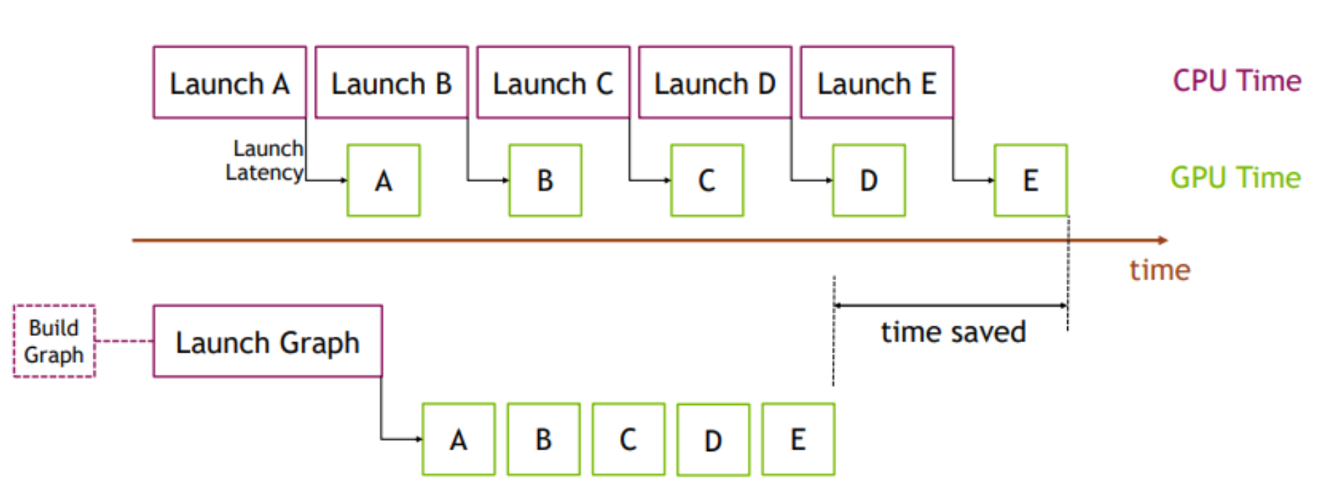
Figure 1. Benefits of using CUDA graphs

NCCL support for CUDA graphs

The previously mentioned benefits of reducing launch overheads also extend to NCCL kernel launches. NCCL enables GPU-based collective and P2P communications. With NCCL support for CUDA graphs, we can eliminate the NCCL kernel launch overhead.

Additionally, kernel launch timing can be unpredictable due to various CPU load and operating system factors. Such time skews can be harmful to the performance of NCCL collective operations. With CUDA graphs, kernels are clustered together so that performance is consistent across ranks in a distributed workload. This is especially useful in large clusters where even a single slow node can bring down overall cluster level performance.

For distributed multi-GPU workloads, NCCL is used for collective communications. If we look at training a neural network that leverages data parallelism, without NCCL support for CUDA graphs, we’ll need a separate launch for each of forward/back propagation and NCCL AllReduce. By contrast, with NCCL support for CUDA graphs, we can reduce launch overhead by lumping together the forward/backward propagation and NCCL AllReduce all in a single graph launch.

With NCCL CUDA graph support, all the kernel launches for NCCL AllReduce for  the forward/backward propagation can be bundled into a graph to reduce overhead launch time.

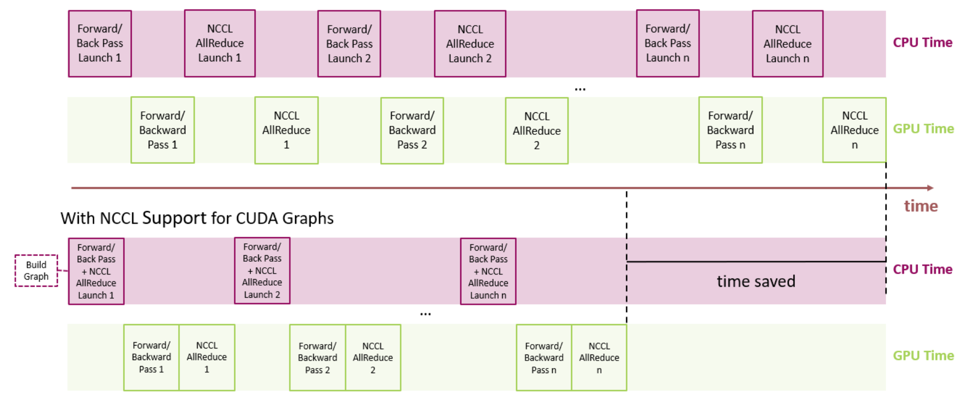
Figure 2. Looking at a typical neural network, all the kernel launches for NCCL AllReduce can be bundled into a graph to reduce overhead launch time.

PyTorch CUDA Graphs

From PyTorch v1.10, the CUDA graphs functionality is made available as a set of beta APIs.

API overview

PyTorch supports the construction of CUDA graphs using stream capture, which puts a CUDA stream in capture mode. CUDA work issued to a capturing stream doesn’t actually run on the GPU. Instead, the work is recorded in a graph. After capture, the graph can be launched to run the GPU work as many times as needed. Each replay runs the same kernels with the same arguments. For pointer arguments this means the same memory addresses are used. By filling input memory with new data (e.g., from a new batch) before each replay, you can rerun the same work on new data.

Replaying a graph sacrifices the dynamic flexibility of typical eager execution in exchange for greatly reduced CPU overhead. A graph’s arguments and kernels are fixed, so a graph replay skips all layers of argument setup and kernel dispatch, including Python, C++, and CUDA driver overheads. Under the hood, a replay submits the entire graph’s work to the GPU with a single call to cudaGraphLaunch. Kernels in a replay also execute slightly faster on the GPU, but eliding CPU overhead is the main benefit.

You should try CUDA graphs if all or part of your network is graph-safe (usually this means static shapes and static control flow, but see the other constraints) and you suspect its runtime is at least somewhat CPU-limited.

API example

PyTorch exposes graphs via a raw torch.cuda.CUDAGraphclass and two convenience wrappers, torch.cuda.graph and torch.cuda.make_graphed_callables.

torch.cuda.graph

torch.cuda.graph is a simple, versatile context manager that captures CUDA work in its context. Before capture, warm up the workload to be captured by running a few eager iterations. Warmup must occur on a side stream. Because the graph reads from and writes to the same memory addresses in every replay, you must maintain long-lived references to tensors that hold input and output data during capture. To run the graph on new input data, copy new data to the capture’s input tensor(s), replay the graph, then read the new output from the capture’s output tensor(s).

If the entire network is capture safe, one can capture and replay the whole network as in the following example.

N, D_in, H, D_out = 640, 4096, 2048, 1024
model = torch.nn.Sequential(torch.nn.Linear(D_in, H),
                            torch.nn.Dropout(p=0.2),
                            torch.nn.Linear(H, D_out),
                            torch.nn.Dropout(p=0.1)).cuda()
loss_fn = torch.nn.MSELoss()
optimizer = torch.optim.SGD(model.parameters(), lr=0.1)

# Placeholders used for capture
static_input = torch.randn(N, D_in, device='cuda')
static_target = torch.randn(N, D_out, device='cuda')

# warmup
# Uses static_input and static_target here for convenience,
# but in a real setting, because the warmup includes optimizer.step()
# you must use a few batches of real data.
s = torch.cuda.Stream()
s.wait_stream(torch.cuda.current_stream())
with torch.cuda.stream(s):
    for i in range(3):
        optimizer.zero_grad(set_to_none=True)
        y_pred = model(static_input)
        loss = loss_fn(y_pred, static_target)
        loss.backward()
        optimizer.step()
torch.cuda.current_stream().wait_stream(s)

# capture
g = torch.cuda.CUDAGraph()
# Sets grads to None before capture, so backward() will create
# .grad attributes with allocations from the graph's private pool
optimizer.zero_grad(set_to_none=True)
with torch.cuda.graph(g):
    static_y_pred = model(static_input)
    # Fills the graph's input memory with new data to compute on
    static_input.copy_(data)
    static_target.copy_(target)
    # replay() includes forward, backward, and step.
    # You don't even need to call optimizer.zero_grad() between iterations
    # because the captured backward refills static .grad tensors in place.
    g.replay()
    # Params have been updated. static_y_pred, static_loss, and .grad
    # attributes hold values from computing on this iteration's data.

If some of your network is unsafe to capture (e.g., due to dynamic control flow, dynamic shapes, CPU syncs, or essential CPU-side logic), you can run the unsafe part(s) eagerly and use torch.cuda.make_graphed_callables() to graph only the capture-safe part(s). This is demonstrated next.

torch.cuda.make_graphed_callables

make_graphed_callables accepts callables (functions or nn.Module and returns graphed versions. By default, callables returned by make_graphed_callables() are autograd-aware, and can be used in the training loop as direct replacements for the functions or nn.Module you passed. make_graphed_callables() internally creates CUDAGraph objects, runs warm up iterations, and maintains static inputs and outputs as needed. Therefore, (unlike with torch.cuda.graph) you don’t need to handle those manually.

In the following example, data-dependent dynamic control flow means the network isn’t capturable end-to-end, but make_graphed_callables() lets us capture and run graph-safe sections as graphs regardless:

N, D_in, H, D_out = 640, 4096, 2048, 1024

module1 = torch.nn.Linear(D_in, H).cuda()
module2 = torch.nn.Linear(H, D_out).cuda()
module3 = torch.nn.Linear(H, D_out).cuda()

loss_fn = torch.nn.MSELoss()
optimizer = torch.optim.SGD(chain(module1.parameters() +
                                  module2.parameters() +
                                  module3.parameters()),
                            lr=0.1)

# Sample inputs used for capture
# requires_grad state of sample inputs must match
# requires_grad state of real inputs each callable will see.
x = torch.randn(N, D_in, device='cuda')
h = torch.randn(N, H, device='cuda', requires_grad=True)

module1 = torch.cuda.make_graphed_callables(module1, (x,))
module2 = torch.cuda.make_graphed_callables(module2, (h,))
module3 = torch.cuda.make_graphed_callables(module3, (h,))

real_inputs = [torch.rand_like(x) for _ in range(10)]
real_targets = [torch.randn(N, D_out, device="cuda") for _ in range(10)]

for data, target in zip(real_inputs, real_targets):
    optimizer.zero_grad(set_to_none=True)

    tmp = module1(data)  # forward ops run as a graph

    if tmp.sum().item() > 0:
        tmp = module2(tmp)  # forward ops run as a graph
    else:
        tmp = module3(tmp)  # forward ops run as a graph

    loss = loss_fn(tmp, y)
    # module2's or module3's (whichever was chosen) backward ops,
    # as well as module1's backward ops, run as graphs
    loss.backward()
    optimizer.step()

Example use cases

MLPerf v1.0 training workloads

The PyTorch CUDA graphs functionality was instrumental in scaling NVIDIA’s MLPerf training v1.0 workloads (implemented in PyTorch) to over 4000 GPUs, setting new records across the board. We illustrate below two MLPerf workloads where the most significant gains were observed with the use of CUDA graphs, yielding up to ~1.7x speedup.

  Number of GPUs Speedup from CUDA-graphs
Mask R-CNN 272 1.70×
BERT 4096 1.12×

Table 1. MLPerf training v1.0 performance improvement with PyTorch CUDA graph.

Mask R-CNN

Deep learning frameworks use GPUs to accelerate computations, but a significant amount of code still runs on CPU cores. CPU cores process meta-data like tensor shapes in order to prepare arguments needed to launch GPU kernels. Processing meta-data is a fixed cost while the cost of the computational work done by the GPUs is positively correlated with batch size. For large batch sizes, CPU overhead is a negligible percentage of total run time cost, but at small batch sizes CPU overhead can become larger than GPU run time. When that happens, GPUs go idle between kernel calls. This issue can be identified on an NSight timeline plot in Figure 3. The plot below shows the “backbone” portion of Mask R-CNN with per-gpu batch size of 1 before graphing. The green portion shows CPU load while the blue portion shows GPU load. In this profile we see that the CPU is maxed out at 100% load while GPU is idle most of the time, there is a lot of empty space between GPU kernels.

NSight timeline plot of Mask R-CNN shows that the CPU is maxed out at 100% load while GPU is idle most of the time, and a lot of empty space between GPU kernels

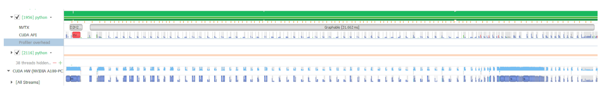
Figure 3: NSight timeline plot of Mask R-CNN

CUDA graphs can automatically eliminate CPU overhead when tensor shapes are static. A complete graph of all the kernel calls is captured during the first step, in subsequent steps the entire graph is launched with a single op, eliminating all the CPU overhead, as observed in Figure 4..

With CUDA graph, the entire graph is launched with a single op, eliminating all the CPU overhead

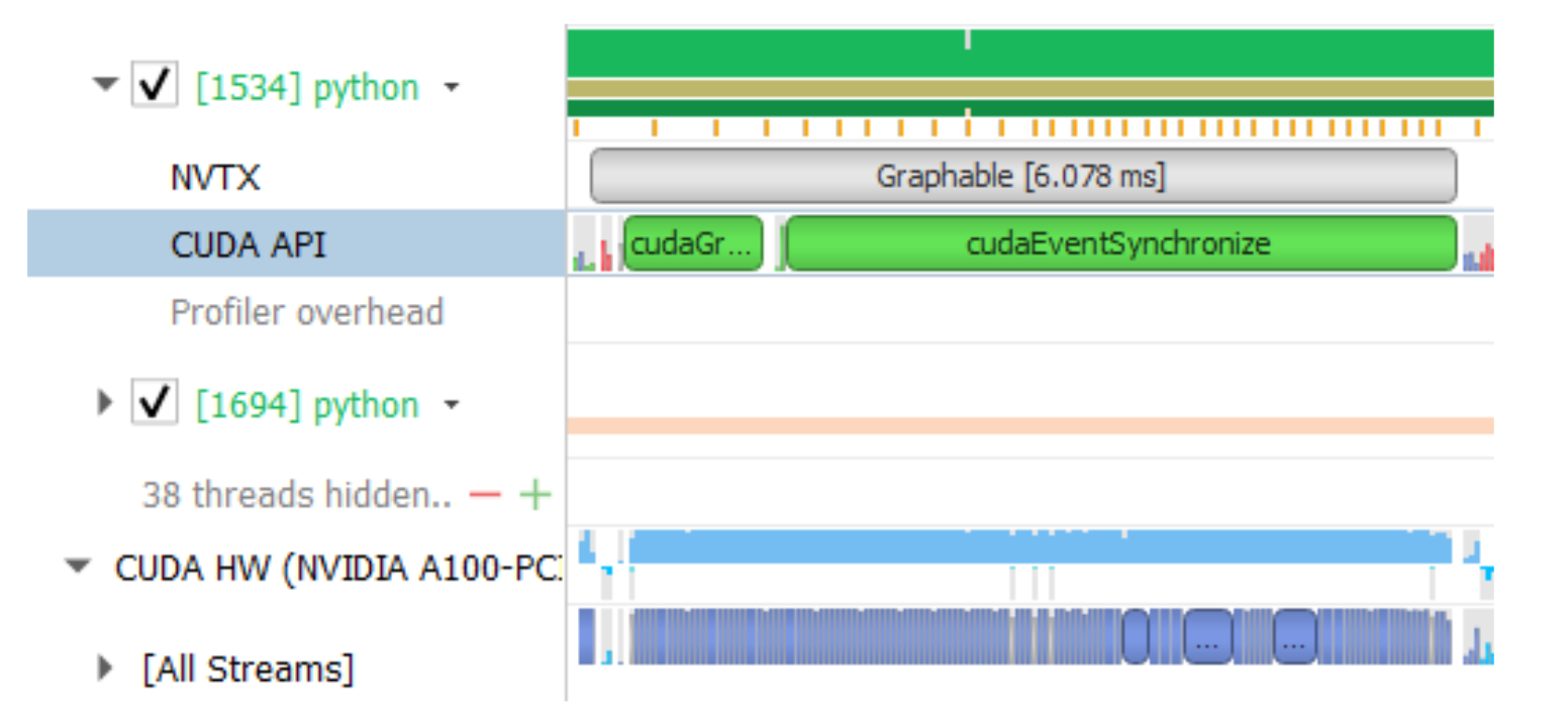
Figure 4: CUDA graphs optimization

With graphing, we see that the GPU kernels are tightly packed and GPU utilization remains high. The graphed portion now runs in 6 ms instead of 31ms, a speedup of 5x. We did not graph the entire model, mostly just the resnet backbone, which resulted in an overall speedup of ~1.7x.
In order to increase the scope of the graph, we made some changes in the software stack to eliminate some of the CPU-GPU synchronization points. In MLPerf v1.0, this work included changing the implementation of torch.randperm function to use CUB instead of Thrust because the latter is a synchronous C++ template library. These improvements are available in the latest NGC container.

BERT

Similarly, by graph capturing the model, we eliminate CPU overhead and accompanying synchronization overhead. CUDA graphs implementation results in a 1.12x performance boost for our max-scale BERT configuration. To maximize the benefits from CUDA graphs, it is important to keep the scope of the graph as large as possible. To achieve this, we modified the model script to remove CPU-GPU synchronizations during the execution such that the full model can be graph captured. Furthermore, we also made sure that the tensor sizes during the execution are static within the scope of the graph. For instance, in BERT, only a specific subset of total tokens contribute to loss function, determined by a pre-generated mask tensor. Extracting the indices of valid tokens from this mask, and using these indices to gather the tokens that contribute to the loss, results in a tensor with a dynamic shape, i.e. with shape that is not constant across iterations. In order to make sure tensor sizes are static, instead of using the dynamic-shape tensors in the loss computation, we used static shape tensors where a mask is used to indicate which elements are valid. As a result, all tensor shapes are static. Dynamic shapes also require CPU-GPU synchronization since it has to involve the framework’s memory management on the CPU side. With static-only shapes, no CPU-GPU synchronizations are necessary. This is shown in Figure 5.

Synchronization free training eliminates CPU synchronization

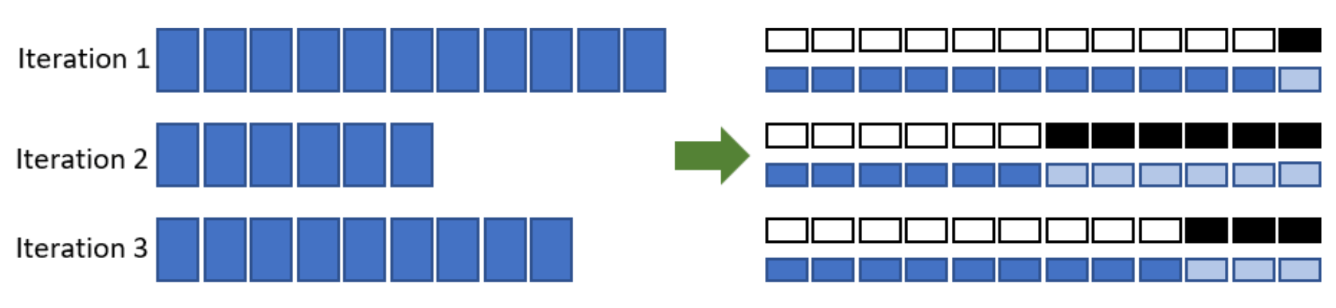
Figure 5. By using a fixed size tensor and a boolean mask as described in the text, we are able to eliminate CPU synchronizations needed for dynamic sized tensors

CUDA graphs in NVIDIA DL examples collection

Single GPU use cases can also benefit from using CUDA Graphs. This is particularly true for workloads launching many short kernels with small batches. A good example is training and inference for recommender systems. Below we present preliminary benchmark results for NVIDIA’s implementation of the Deep Learning Recommendation Model (DLRM) from our Deep Learning Examples collection. Using CUDA graphs for this workload provides significant speedups for both training and inference. The effect is particularly visible when using very small batch sizes, where CPU overheads are more pronounced.

CUDA graphs are being actively integrated into other PyTorch NGC model scripts and the NVIDIA Github deep learning examples. Stay tuned for more examples on how to use it.

CUDA graphs optimization for the DLRM model. The impact is larger for smaller batch sizes where CPU overheads are more pronounced.

CUDA graphs optimization for the DLRM model. The impact is larger for smaller batch sizes where CPU overheads are more pronounced.

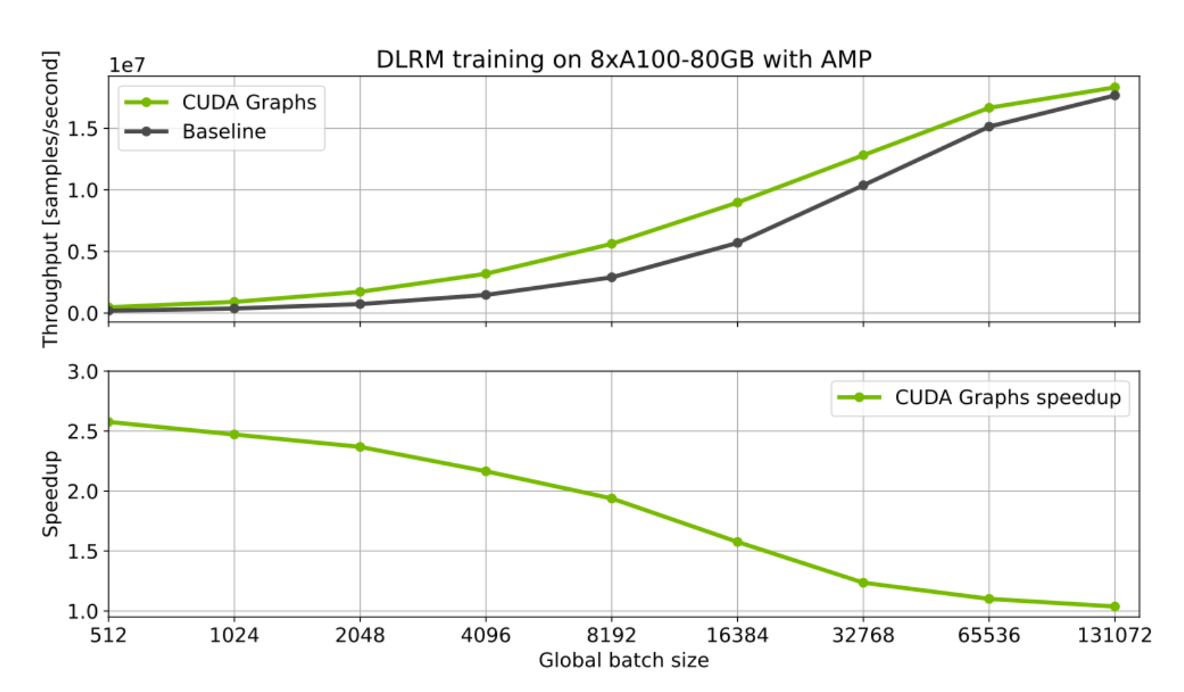
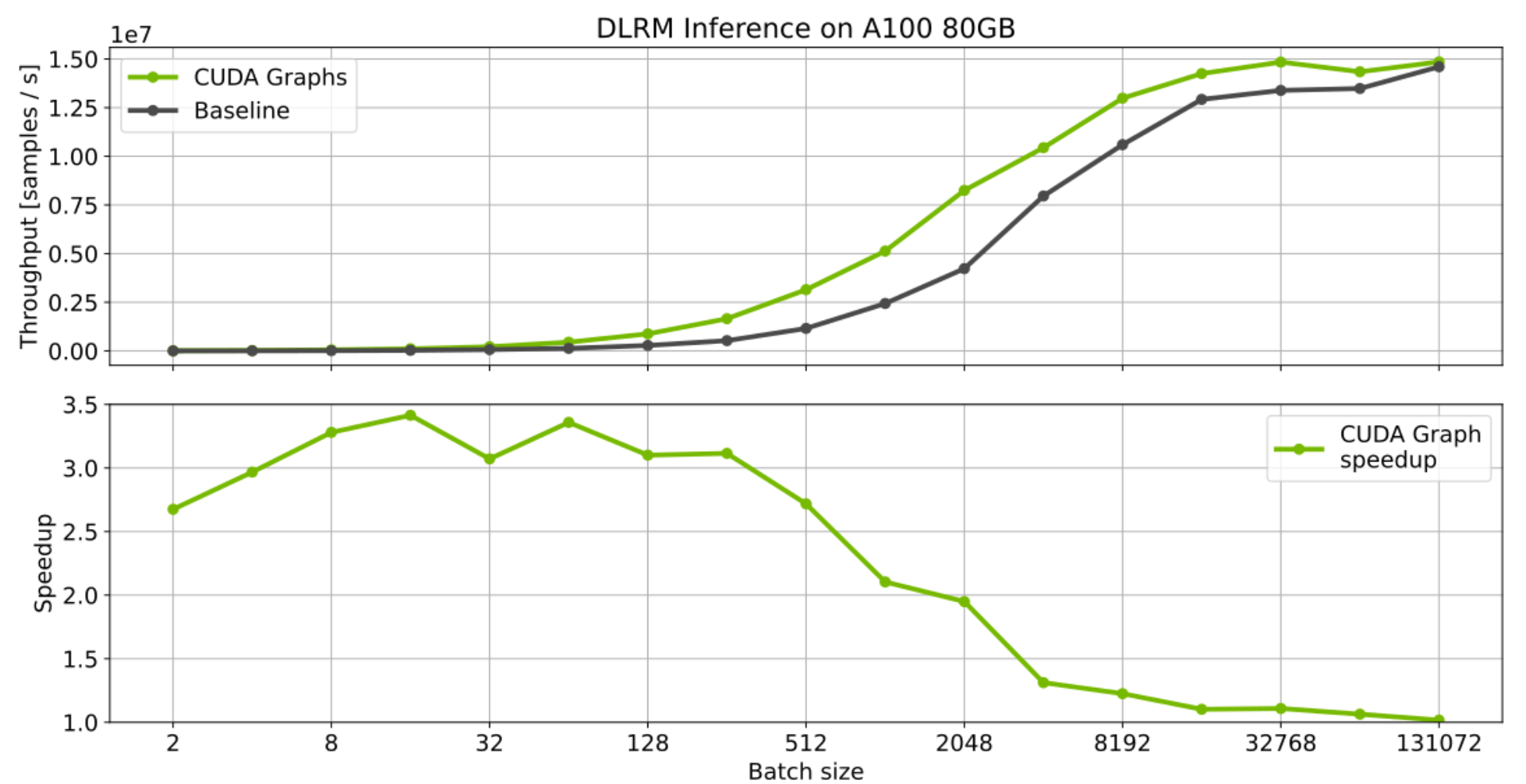
Figure 6: CUDA graphs optimization for the DLRM model.

Call to action: CUDA Graphs in PyTorch v1.10

CUDA graphs can provide substantial benefits for workloads that comprise many small GPU kernels and hence bogged down by CPU launch overheads. This has been demonstrated in our MLPerf efforts, optimizing PyTorch models. Many of these optimizations, including CUDA graphs, have or will eventually be integrated into our PyTorch NGC model scripts collection and the NVIDIA Github deep learning examples. For now, check out our open-source MLPerf training v1.0 implementation which could serve as a good starting point to see CUDA graph in action. Alternatively, try the PyTorch CUDA graphs API on your own workloads.

We thank many NVIDIAN’s and Facebook engineers for their discussions and suggestions:
Karthik Mandakolathur US,
Tomasz Grel,
PLJoey Conway,
Arslan Zulfiqar US

Authors bios

Vinh Nguyen
DL Engineer, NVIDIA

Vinh is a Deep learning engineer and data scientist, having published more than 50 scientific articles attracting more than 2500 citations. At NVIDIA, his work spans a wide range of deep learning and AI applications, including speech, language and vision processing, and recommender systems.

Michael Carilli
Senior Developer Technology Engineer, NVIDIA

Michael worked at the Air Force Research Laboratory optimizing CFD code for modern parallel architectures. He holds a PhD in computational physics from the University of California, Santa Barbara. A member of the PyTorch team, he focuses on making GPU training fast, numerically stable, and easy(er) for internal teams, external customers, and Pytorch community users.

Sukru Burc Eryilmaz
Senior Architect in Dev Arch, NVIDIA

Sukru received his PhD from Stanford University, and B.S from Bilkent University. He currently works on improving the end-to-end performance of neural network training both at single-node scale and supercomputer scale.

Vartika Singh
Tech Partner Lead for DL Frameworks and Libraries, NVIDIA

Vartika has led teams working in confluence of cloud and distributed computing, scaling and AI, influencing the design and strategy of major corporations. She currently works with the major frameworks and compiler organizations and developers within and outside NVIDIA, to help the design to work efficiently and optimally on NVIDIA hardware.

Michelle Lin
Product Intern, NVIDIA

Michelle is currently pursuing an undergraduate degree in Computer Science and Business Administration at UC Berkeley. She is currently managing execution of projects such as conducting market research and creating marketing assets for Magnum IO.

Natalia Gimelshein
Applied Research Scientist, Facebook

Natalia Gimelshein worked on GPU performance optimization for deep learning workloads at NVIDIA and Facebook. She is currently a member of the PyTorch core team, working with partners to seamlessly support new software and hardware features.

Alban Desmaison
Research Engineer, Facebook

Alban studied engineering and did a PhD in Machine Learning and Optimization, during which he was an OSS contributor to PyTorch prior to joining Facebook. His main responsibilities are maintaining some core library and features (autograd, optim, nn) and working on making PyTorch better in general.

Edward Yang
Research Engineer, Facebook

Edward studied CS at MIT and then Stanford before starting at Facebook. He is a part of the PyTorch core team and is one of the leading contributors to PyTorch.

Read More

Artificial intelligence sheds light on how the brain processes language

In the past few years, artificial intelligence models of language have become very good at certain tasks. Most notably, they excel at predicting the next word in a string of text; this technology helps search engines and texting apps predict the next word you are going to type.

The most recent generation of predictive language models also appears to learn something about the underlying meaning of language. These models can not only predict the word that comes next, but also perform tasks that seem to require some degree of genuine understanding, such as question answering, document summarization, and story completion. 

Such models were designed to optimize performance for the specific function of predicting text, without attempting to mimic anything about how the human brain performs this task or understands language. But a new study from MIT neuroscientists suggests the underlying function of these models resembles the function of language-processing centers in the human brain.

Computer models that perform well on other types of language tasks do not show this similarity to the human brain, offering evidence that the human brain may use next-word prediction to drive language processing.

“The better the model is at predicting the next word, the more closely it fits the human brain,” says Nancy Kanwisher, the Walter A. Rosenblith Professor of Cognitive Neuroscience, a member of MIT’s McGovern Institute for Brain Research and Center for Brains, Minds, and Machines (CBMM), and an author of the new study. “It’s amazing that the models fit so well, and it very indirectly suggests that maybe what the human language system is doing is predicting what’s going to happen next.”

Joshua Tenenbaum, a professor of computational cognitive science at MIT and a member of CBMM and MIT’s Artificial Intelligence Laboratory (CSAIL); and Evelina Fedorenko, the Frederick A. and Carole J. Middleton Career Development Associate Professor of Neuroscience and a member of the McGovern Institute, are the senior authors of the study, which appears this week in the Proceedings of the National Academy of Sciences. Martin Schrimpf, an MIT graduate student who works in CBMM, is the first author of the paper.

Making predictions

The new, high-performing next-word prediction models belong to a class of models called deep neural networks. These networks contain computational “nodes” that form connections of varying strength, and layers that pass information between each other in prescribed ways.

Over the past decade, scientists have used deep neural networks to create models of vision that can recognize objects as well as the primate brain does. Research at MIT has also shown that the underlying function of visual object recognition models matches the organization of the primate visual cortex, even though those computer models were not specifically designed to mimic the brain.

In the new study, the MIT team used a similar approach to compare language-processing centers in the human brain with language-processing models. The researchers analyzed 43 different language models, including several that are optimized for next-word prediction. These include a model called GPT-3 (Generative Pre-trained Transformer 3), which, given a prompt, can generate text similar to what a human would produce. Other models were designed to perform different language tasks, such as filling in a blank in a sentence.

As each model was presented with a string of words, the researchers measured the activity of the nodes that make up the network. They then compared these patterns to activity in the human brain, measured in subjects performing three language tasks: listening to stories, reading sentences one at a time, and reading sentences in which one word is revealed at a time. These human datasets included functional magnetic resonance (fMRI) data and intracranial electrocorticographic measurements taken in people undergoing brain surgery for epilepsy.

They found that the best-performing next-word prediction models had activity patterns that very closely resembled those seen in the human brain. Activity in those same models was also highly correlated with measures of human behavioral measures such as how fast people were able to read the text.

“We found that the models that predict the neural responses well also tend to best predict human behavior responses, in the form of reading times. And then both of these are explained by the model performance on next-word prediction. This triangle really connects everything together,” Schrimpf says.

“A key takeaway from this work is that language processing is a highly constrained problem: The best solutions to it that AI engineers have created end up being similar, as this paper shows, to the solutions found by the evolutionary process that created the human brain. Since the AI network didn’t seek to mimic the brain directly — but does end up looking brain-like — this suggests that, in a sense, a kind of convergent evolution has occurred between AI and nature,” says Daniel Yamins, an assistant professor of psychology and computer science at Stanford University, who was not involved in the study.

Game changer

One of the key computational features of predictive models such as GPT-3 is an element known as a forward one-way predictive transformer. This kind of transformer is able to make predictions of what is going to come next, based on previous sequences. A significant feature of this transformer is that it can make predictions based on a very long prior context (hundreds of words), not just the last few words.

Scientists have not found any brain circuits or learning mechanisms that correspond to this type of processing, Tenenbaum says. However, the new findings are consistent with hypotheses that have been previously proposed that prediction is one of the key functions in language processing, he says.

“One of the challenges of language processing is the real-time aspect of it,” he says. “Language comes in, and you have to keep up with it and be able to make sense of it in real time.”

The researchers now plan to build variants of these language processing models to see how small changes in their architecture affect their performance and their ability to fit human neural data.

“For me, this result has been a game changer,” Fedorenko says. “It’s totally transforming my research program, because I would not have predicted that in my lifetime we would get to these computationally explicit models that capture enough about the brain so that we can actually leverage them in understanding how the brain works.”

The researchers also plan to try to combine these high-performing language models with some computer models Tenenbaum’s lab has previously developed that can perform other kinds of tasks such as constructing perceptual representations of the physical world.

“If we’re able to understand what these language models do and how they can connect to models which do things that are more like perceiving and thinking, then that can give us more integrative models of how things work in the brain,” Tenenbaum says. “This could take us toward better artificial intelligence models, as well as giving us better models of how more of the brain works and how general intelligence emerges, than we’ve had in the past.”

The research was funded by a Takeda Fellowship; the MIT Shoemaker Fellowship; the Semiconductor Research Corporation; the MIT Media Lab Consortia; the MIT Singleton Fellowship; the MIT Presidential Graduate Fellowship; the Friends of the McGovern Institute Fellowship; the MIT Center for Brains, Minds, and Machines, through the National Science Foundation; the National Institutes of Health; MIT’s Department of Brain and Cognitive Sciences; and the McGovern Institute.

Other authors of the paper are Idan Blank PhD ’16 and graduate students Greta Tuckute, Carina Kauf, and Eghbal Hosseini.

Read More

Deciding Which Tasks Should Train Together in Multi-Task Neural Networks

Posted by Christopher Fifty, Research Engineer, Google Research, Brain Team

Many machine learning (ML) models typically focus on learning one task at a time. For example, language models predict the probability of a next word given a context of past words, and object detection models identify the object(s) that are present in an image. However, there may be instances when learning from many related tasks at the same time would lead to better modeling performance. This is addressed in the domain of multi-task learning, a subfield of ML in which multiple objectives are trained within the same model at the same time.

Consider a real-world example: the game of ping-pong. When playing ping-pong, it is often advantageous to judge the distance, spin, and imminent trajectory of the ping-pong ball to adjust your body and line up a swing. While each of these tasks are unique — predicting the spin of a ping-pong ball is fundamentally distinct from predicting its location — improving your reasoning of the location and spin of the ball will likely help you better predict its trajectory and vice-versa. By analogy, within the realm of deep learning, training a model to predict three related tasks (i.e., the location, spin, and trajectory of a ping-pong ball) may result in improved performance over a model that only predicts a single objective.

Left: Three single-task networks, each of which uses the same input to predict the spin, distance, or trajectory of the ping-pong ball, respectively. Right: A single multi-task network that simultaneously predicts the spin, distance, and trajectory.

In “Efficiently Identifying Task Groupings in Multi-Task Learning”, a spotlight presentation at NeurIPS 2021, we describe a method called Task Affinity Groupings (TAG) that determines which tasks should be trained together in multi-task neural networks. Our approach attempts to divide a set of tasks into smaller subsets such that the performance across all tasks is maximized. To accomplish this goal, it trains all tasks together in a single multi-task model and measures the degree to which one task’s gradient update on the model’s parameters would affect the loss of the other tasks in the network. We denote this quantity as inter-task affinity. Our experimental findings indicate that selecting groups of tasks that maximize inter-task affinity correlates strongly with overall model performance.

Which Tasks Should Train Together?
In the ideal case, a multi-task learning model will apply the information it learns during training on one task to decrease the loss on other tasks included in training the network. This transfer of information leads to a single model that can not only make multiple predictions, but may also exhibit improved accuracy for those predictions when compared with the performance of training a different model for each task. On the other hand, training a single model on many tasks may lead to competition for model capacity and severely degrade performance. This latter scenario often occurs when tasks are unrelated. Returning to our ping-pong analogy, imagine trying to predict the location, spin, and trajectory of the ping-pong ball while simultaneously recounting the Fibonnaci sequence. Not a fun prospect, and most likely detrimental to your progression as a ping-pong player.

One direct approach to select the subset of tasks on which a model should train is to perform an exhaustive search over all possible combinations of multi-task networks for a set of tasks. However, the cost associated with this search can be prohibitive, especially when there are a large number of tasks, because the number of possible combinations increases exponentially with respect to the number of tasks in the set. This is further complicated by the fact that the set of tasks to which a model is applied may change throughout its lifetime. As tasks are added to or dropped from the set of all tasks, this costly analysis would need to be repeated to determine new groupings. Moreover, as the scale and complexity of models continues to increase, even approximate task grouping algorithms that evaluate only a subset of possible multi-task networks may become prohibitively costly and time-consuming to evaluate.

Building Task Affinity Groupings
In examining this challenge, we drew inspiration from meta-learning, a domain of machine learning that trains a neural network that can be quickly adapted to a new, and previously unseen task. One of the classic meta-learning algorithms, MAML, applies a gradient update to the models’ parameters for a collection of tasks and then updates its original set of parameters to minimize the loss for a subset of tasks in that collection computed at the updated parameter values. Using this method, MAML trains the model to learn representations that will not minimize the loss for its current set of weights, but rather for the weights after one or more steps of training. As a result, MAML trains a models’ parameters to have the capacity to quickly adapt to a previously unseen task because it optimizes for the future, not the present.

TAG employs a similar mechanism to gain insight into the training dynamics of multi-task neural networks. In particular, it updates the model’s parameters with respect only to a single task, looks at how this change would affect the other tasks in the multi-task neural network, and then undoes this update. This process is then repeated for every other task to gather information on how each task in the network would interact with any other task. Training then continues as normal by updating the model’s shared parameters with respect to every task in the network.

Collecting these statistics, and looking at their dynamics throughout training, reveals that certain tasks consistently exhibit beneficial relationships, while some are antagonistic towards each other. A network selection algorithm can leverage this data in order to group tasks together that maximize inter-task affinity, subject to a practitioner’s choice of how many multi-task networks can be used during inference.

Overview of TAG. First, tasks are trained together in the same network while computing inter-task affinities. Second, the network selection algorithm finds task groupings that maximize inter-task affinity. Third, the resulting multi-task networks are trained and deployed.

Results
Our experimental findings indicate that TAG can select very strong task groupings. On the CelebA and Taskonomy datasets, TAG is competitive with the prior state-of-the-art, while operating between 32x and 11.5x faster, respectively. On the Taskonomy dataset, this speedup translates to 2,008 fewer Tesla V100 GPU hours to find task groupings.

Conclusion
TAG is an efficient method to determine which tasks should train together in a single training run. The method looks at how tasks interact through training, notably, the effect that updating the model’s parameters when training on one task would have on the loss values of the other tasks in the network. We find that selecting groups of tasks to maximize this score correlates strongly with model performance.

Acknowledgements
We would like to thank Ehsan Amid, Zhe Zhao, Tianhe Yu, Rohan Anil, and Chelsea Finn for their fundamental contributions to this work. We also recognize Tom Small for designing the animation, and Google Research as a whole for fostering a collaborative and uplifting research environment.

Read More

Designs from Data: Offline Black-Box Optimization via Conservative Training

<!– –>


Figure 1: Offline Model-Based Optimization (MBO): The goal of offline MBO is to optimize an unknown objective function $f(x)$ with respect to $x$, provided access to only as static, previously-collected dataset of designs.

Machine learning methods have shown tremendous promise on prediction problems: predicting the efficacy of a drug, predicting how a protein will fold, or predicting the strength of a composite material. But can we use machine learning for design? Conventionally, such problems have been tackled with black-box optimization procedures that repeatedly query an objective function. For instance, if designing a drug, the algorithm will iteratively modify the drug, test it, then modify it again. But when evaluating the efficacy of a candidate design involves conducting a real-world experiment, this can quickly become prohibitive. An appealing alternative is to create designs from data. Instead of requiring active synthesis and querying, can we devise a method that simply examines a large dataset of previously tested designs (e.g., drugs that have been evaluated before), and comes up with a new design that is better? We call this offline model-based optimization (offline MBO), and in this post, we discuss offline MBO methods and some recent advances.

A First-Principles Theory of NeuralNetwork Generalization


Fig 1. Measures of generalization performance for neural networks trained on four different boolean functions (colors) with varying training set size. For both MSE (left) and learnability (right), theoretical predictions (curves) closely match true performance (dots).

Deep learning has proven a stunning success for countless problems of interest, but this success belies the fact that, at a fundamental level, we do not understand why it works so well. Many empirical phenomena, well-known to deep learning practitioners, remain mysteries to theoreticians. Perhaps the greatest of these mysteries has been the question of generalization: why do the functions learned by neural networks generalize so well to unseen data? From the perspective of classical ML, neural nets’ high performance is a surprise given that they are so overparameterized that they could easily represent countless poorly-generalizing functions.