Monthly Archives: January 2021

In this post, we walk you through the steps to build machine learning (ML) models in Amazon SageMaker with data stored in Amazon HealthLake using two example predictive disease models we trained on sample data using the MIMIC-III dataset. This dataset was developed by the MIT lab for Computational Physiology and consists of de-identified healthcare data associated with approximately 60,000 ICU admissions. The dataset includes multiple attributes about the patients like their demographics, vital signs, and medications, along with their clinical notes. We first developed the models using the structured data such as demographics, vital signs, and medications. Then we augmented these models with additional data extracted and normalized from clinical notes to test and compare their performance. In both these experiments, we found an improvement in model performance when modelled as a supervised learning (classification) or an unsupervised learning (clustering) problem. We present our findings and the setup of the experiments in this post.

Why multiple modalities?

Modality can be defined as the classification of a single independent sensory input/output between a computer and a human. For example, we can see objects and hear sounds by using our senses. These can be considered as two separate modalities. Datasets that represent multiple modalities are categorized as a multi-modal dataset. For instance, images can consist of tags that help search and organize them, and textual data can contain images to explain what’s in the image. When medical practitioners make clinical decisions, it’s usually based on information gathered from a variety of healthcare data modalities. A physician looks at patient’s observations, their past history, their scans, and even physical characteristics of the patient during the visit to make a definitive diagnosis. ML models need to take this into account when trying to achieve real-world performance. The post Building a medical image search platform on AWS shows how you can combine features from medical images and their corresponding radiology reports to create a medical image search platform. The challenge with creating such models is the preprocessing of these multi-modal datasets and extracting appropriate features from them.

Amazon HealthLake makes it easier to train models on multi-modal data

Amazon HealthLake is a HIPAA eligible service that enables healthcare providers, health insurance companies, and pharmaceutical companies to store, transform, query, and analyze health data on the AWS Cloud at petabyte scale. As part of the transformation, Amazon HealthLake tags and indexes unstructured data using specialized ML models. These tags and indexes can be used to query and search as well as understand relationships in the data for analytics.

When you export data from Amazon HealthLake, it adds a resource called DocumentReference to the output. This resource consists of clinical entities (Like medications, medical conditions, anatomy, and Protected Health Information (PHI)), the RxNorm codes for medications, and the ICD10 codes for medical conditions that are automatically derived from the unstructured notes about the patients. These are additional attributes about the patients that are embedded within the unstructured portions of their clinical records and would have been largely ignored for downstream analysis. Combining the structured data from the EHR with these attributes provides a more holistic picture of the patient and their conditions. To help determine the value of these attributes, we created a couple of experiments around clinical outcome prediction.

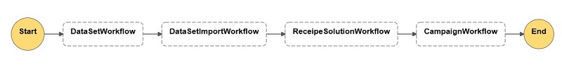
Architecture overview

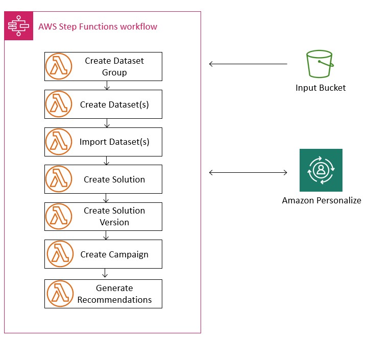
The following diagram illustrates the architecture for our experiments.

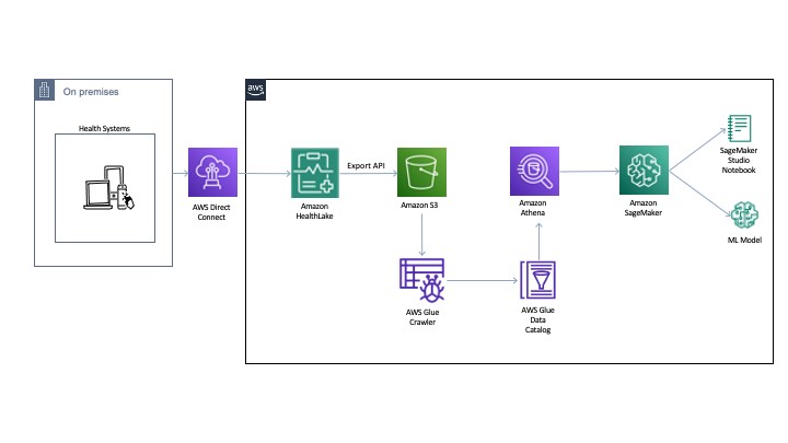
You can export the normalized data to an Amazon Simple Storage Service (Amazon S3) bucket using the Export API. Then we use AWS Glue to crawl and build a catalog of the data. This catalog is shared by Amazon Athena to run the queries directly off of the exported data from Colossus. Athena also normalizes the JSON format files to rows and columns for easy querying. The DocumentReference resource JSON file is processed separately to extract indexed data derived from the unstructured portions of the patient records. The file consists of an extension tag that has a hierarchical JSON output consisting of patient attributes. There are multiple ways to process this file (like using Python-based JSON parsers or even string-based regex and pattern matching). For an example implementation, see the section Connecting Athena with HealthLake in the post Population health applications with Amazon HealthLake – Part 1: Analytics and monitoring using Amazon QuickSight.

Example setup

Accessing the MIMIC-III dataset requires you to request access. As part of this post, we don’t distribute any data but instead provide the setup steps so you can replicate these experiments when you have access to MIMIC-III. We also publish our conclusions and findings from the results.

For the first experiment, we build a binary disease classification model to predict patients with congestive heart failure (CHF). We measure its performance using accuracy, ROC, and confusion matrix for both structured and unstructured patient records. For the second experiment, we cluster a cohort of patients into a fixed number of groups and visualize the cluster separation before and after the addition of the unstructured patient records. For both our experiments, we build a baseline model and compare it with the multi-modal model, where we combine existing structured data with additional features (ICD-10 codes and Rx-Norm codes) in our training set.

These experiments are not intended to produce a state-of-the-art model on real-world datasets; its purpose is to demonstrate how you can utilize features exported from Amazon Healthlake for training models on structured and unstructured patient records to improve your overall model performance.

Features and data normalization

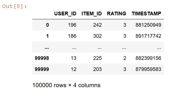
We took a variety of features related to patient encounters to train our models. This included the patient demographics (gender, marital status), the clinical conditions, procedures, medications, and observations. Because each patient could have multiple encounters consisting of multiple observations, clinical conditions, procedures, and medications, we normalized the data and converted each of these features into a list. This allowed us to get a training set with all these features (as a list) for each patient.

Similarly, for the unstructured features that Amazon Healthlake converted into the DocumentReference resource, we extracted the ICD-10 codes and Rx-Norm codes (using the methods described in the architecture) and converted them into feature vectors.

Feature engineering and model

For the categorical attributes in our dataset, we used a label encoder to convert the attributes into a numerical representation. For all other list attributes, we used term frequency-inverse document frequency (FI-IDF) vectors. This high-dimensional dataset was then shuffled and divided into 80% train and 20% test sets for training and evaluation of the models, respectively. For training our model, we used the gradient boosting library XGBoost. We considered mostly default hyperparameters and didn’t perform any hyperparameter tuning, because our objective was only to train a baseline model with structured patient records and then show improvement on those results with the unstructured features. Adopting better hyperparameters or changing to other feature engineering and modelling approaches can likely improve these results.

Example 1: Predicting patients with a congestive heart failure

For the first experiment, we took 500 patients with a positive CHF diagnosis. For the negative class, we randomly selected 500 patients who didn’t have a CHF diagnosis. We removed the clinical conditions from the positive class of patients that were directly related to CHF. For example, all the patients in the positive class were expected to have ICD-9 code 428, which stands for CHF. We filtered that out from the positive class to make sure the model is not overfitting on the clinical condition.

Baseline model

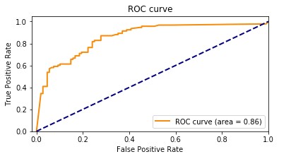
Our baseline model had an accuracy of 85.8%. The following graph shows the ROC curve.

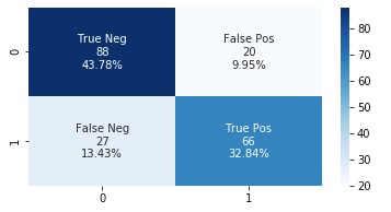
The following graph shows the confusion matrix.

Amazon HealthLake augmented model

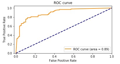
Our Amazon HealthLake augmented model had an accuracy of 89.1%. The following graph shows the ROC curve.

The following graph shows the confusion matrix.

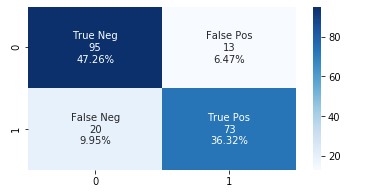
Adding the features extracted from Amazon HealthLake allowed us to improve the model accuracy from 85% to 89% and also the AUC from 0.86 to 0.89. If you look at the confusion matrices for the two models, the false positives reduced from 20 to 13 and the false negatives reduced from 27 to 20.

Optimizing healthcare is about ensuring the patient is associated with their peers and the right cohort. As patient data is added or changes, it’s important to continuously identify and reduce false negative and positive identifiers for overall improvement in the quality of care.

To better explain the performance improvements, we picked a patient from the false negative cohort in the first model who moved to true positive in the second model. We plotted a word cloud for the top medical conditions for this patient for the first and the second model, as shown in the following images.

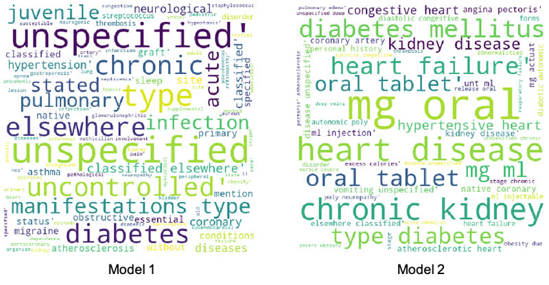
There is a clear difference between the medical conditions of the patient before and after the addition of features from Amazon HealthLake. The word cloud for model 2 is richer, with more medical conditions indicative of CHF than the one for model 1. The data embedded within the unstructured notes for this patient extracted by Amazon HealthLake helped this patient move from a false negative category to a true positive.

These numbers are based on synthetic experimental data we used from a subset of MIMIC-III patients. In a real-world scenario with higher-volume of patients, these numbers may differ.

Example 2: Grouping patients diagnosed with sepsis

For the second experiment, we took 500 patients with a positive sepsis diagnosis. We grouped these patients on the basis of their structured clinical records using k-means clustering. To show that this is a repeatable pattern, we chose the same feature engineering techniques as described in experiment 1. We didn’t divide the data into training and testing datasets because we were implementing an unsupervised learning algorithm.

We first analyzed the optimal number of clusters of the grouping using the Elbow method and arrived at the curve shown in the following graph.

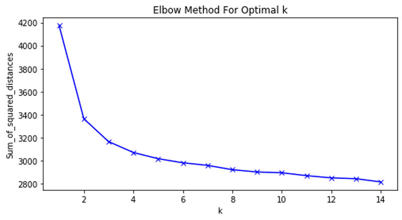
This allowed us to determine that six clusters were the optimal number in our patient grouping.

Baseline model

We reduced the dimensionality of the input data using Principal Component Analysis (PCA) to two and plotted the following scatter plot.

The following were the counts of patients across each cluster:

Cluster 1
Number of patients: 44

Cluster 2
Number of patients: 30

Cluster 3
Number of patients: 109

Cluster 4
Number of patients: 66

Cluster 5
Number of patients: 106

Cluster 6
Number of patients: 145

We found that the at least four of the six clusters had a distinct overlap of patients. That means the structured clinical features weren’t enough to clearly divide the patients into six groups.

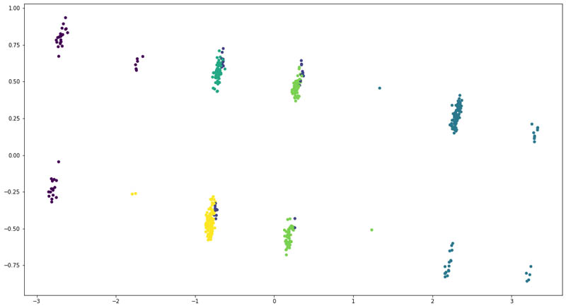
Enhanced model

For the enhanced model, we added the ICD-10 codes and their corresponding descriptions for each patient as extracted from Amazon HealthLake. However, this time, we could see a clear separation of the patient groups.

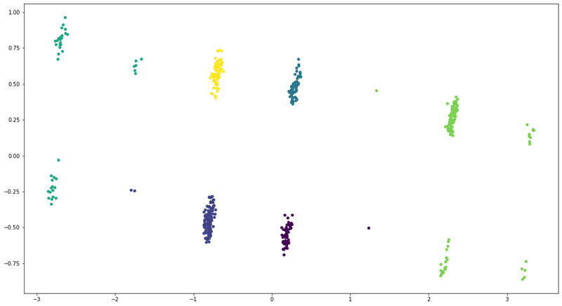
We also saw a change in distribution across the six clusters:

Cluster 1
Number of patients: 54

Cluster 2
Number of patients: 154

Cluster 3
Number of patients: 64

Cluster 4
Number of patients: 44

Cluster 5
Number of patients: 109

Cluster 6
Number of patients: 75

As you can see, adding features from the unstructured data for the patients allows us to improve the clustering model to clearly divide the patients into six clusters. We even saw that some patients moved across clusters, denoting that the model became better at recognizing those patients based on their unstructured clinical records.

Conclusion

In this post, we demonstrated how you can easily use SageMaker to build ML models on your data in Amazon HealthLake. We also demonstrated the advantages of augmenting data from unstructured clinical notes to improve the accuracy of disease prediction models. We hope this body of work provides you with examples of how to build ML models using SageMaker with your data stored and normalized in Amazon HealthLake and improve model performance for clinical outcome predictions. To learn more about Amazon HealthLake, please check the website and technical documentation for more information.

About the Authors

Ujjwal Ratan is a Principal Machine Learning Specialist in the Global Healthcare and Lifesciences team at Amazon Web Services. He works on the application of machine learning and deep learning to real world industry problems like medical imaging, unstructured clinical text, genomics, precision medicine, clinical trials and quality of care improvement. He has expertise in scaling machine learning/deep learning algorithms on the AWS cloud for accelerated training and inference. In his free time, he enjoys listening to (and playing) music and taking unplanned road trips with his family.

Nihir Chadderwala is an AI/ML Solutions Architect on the Global Healthcare and Life Sciences team. His background is building Big Data and AI-powered solutions to customer problems in variety of domains such as software, media, automotive, and healthcare. In his spare time, he enjoys playing tennis, watching and reading about Cosmos.

Parminder Bhatia is a science leader in the AWS Health AI, currently building deep learning algorithms for clinical domain at scale. His expertise is in machine learning and large scale text analysis techniques in low resource settings, especially in biomedical, life sciences and healthcare technologies. He enjoys playing soccer, water sports and traveling with his family.

Read More

Machine learning (ML)-based recommender systems aren’t a new concept across organizations such as retail, media and entertainment, and education, but developing such a system can be a resource-intensive task—from data labelling, training and inference, to scaling. You also need to apply continuous integration, continuous deployment, and continuous training to your ML model, or MLOps. The MLOps model helps build code and integration across ML tools and frameworks. Moreover, building a recommender system requires managing and orchestrating multiple workflows, for example waiting for your training jobs to finish and trigger deployments.

In this post, we show you how to use Amazon Personalize to create a serverless recommender system for movie recommendations with no ML experience required. Creating an Amazon Personalize solution workflow involves multiple steps, such as preparing and importing the data, choosing a recipe and creating a solution and finally generating recommendations. End-users or your data scientists can orchestrate these steps using AWS Lambda functions and AWS Step Functions. However, writing JSON code to manage such workflows can be complicated for your data scientists.

You can orchestrate an Amazon Personalize workflow using the AWS Step Functions Data Science SDK for Python using an Amazon SageMaker Jupyter notebook. The AWS Step Functions Data Science SDK is an open-source library that allows data scientists to easily create workflows that process and publish ML models using Amazon SageMaker Jupyter notebooks and Step Functions. You can create multi-step ML workflows in Python that orchestrate AWS infrastructure at scale, without having to provision and integrate the AWS services separately.

Solution and services overview

We have orchestrated the Amazon Personalize training workflow steps such as preparing and importing the data, choosing a recipe and creating a solution using AWS Step functions and AWS lambda functions to create a below Amazon Personalize end to end automated workflow:

We walk you through the below steps using the accompanying Amazon SageMaker Jupyter notebook. In order to create the above Amazon Personalize workflow, we are going to follow below detailed steps:

1. Complete the prerequisites of setting up permissions and preparing the dataset.
2. Set up AWS Lambda function and AWS Step function task states.
3. Add wait conditions to each AWS Step function task states.
4. Add a control flow and link the states.
5. Define and run the workflows by combining all the above steps.
6. Generate recommendations.

Prerequisites

Before you build your workflow and generate recommendations, you must set up a notebook instance, AWS Identity and Access Management (IAM) roles, and create an Amazon Simple Storage Service (Amazon S3) bucket.

Creating a notebook instance in Amazon SageMaker

Create an Amazon SageMaker notebook Instance by following instructions here. For creating IAM role for your notebook, make sure your notebook IAM role has AmazonS3FullAccess and AmazonPersonalizeFullAccess in order to access Amazon S3 and Amazon Personalize APIs through the Sagemaker notebook.

1. When the notebook is active, choose Open Jupyter.
2. On the Jupyter dashboard, choose New.
3. Choose Terminal.
4. In the terminal, enter the following code:

   cd SageMaker 
   git clone https://github.com/aws-samples/personalize-data-science-sdk-workflow.git

5. Open the notebook by choosing Personalize-Stepfunction-Workflow.ipynb in the root folder.

You’re now ready to run the following steps through the notebook cells. You can find the complete notebook for this solution in the GitHub repo.

Setting up Step Function Execution role

You need a Step Functions execution role so that you can create and invoke workflows in Step Functions. For instructions, see Create a role for Step Functions or go through the steps in the notebook Create an execution role for Step Functions.

Attach an inline policy to the role you created for notebook instance in previous step. Enter the JSON policy by copying the policy from the notebook.

Preparing your dataset

To prepare your dataset, complete the following steps:

1. Create an S3 bucket to store the training dataset and provide the bucket name and file name as ’movie-lens-100k.csv’ in the notebook step Setup S3 location and filename. See the following code:

   bucket = "<SAMPLE BUCKET NAME>" # replace with the name of your S3 bucket
   filename = "<SAMPLE FILE NAME>" # replace with a name that you want to save the dataset under

2. Attach the policy to the S3 bucket by running the Attach policy to Amazon S3 bucket step in the notebook.
3. Create an IAM role for Amazon Personalize by running the Create Personalize Role step in the notebook using Python boto3 create_role API.

4. To preprocess the dataset and upload to Amazon S3, run the Data-Preparation step of the following notebook cell to download the movie-lens dataset and select the movies that have a rating of 2 or above from the dataset:

   !wget -N http://files.grouplens.org/datasets/movielens/ml-100k.zip
   !unzip -o ml-100k.zip
   data = pd.read_csv('./ml-100k/u.data', sep='t', names=['USER_ID', 'ITEM_ID', 'RATING', 'TIMESTAMP'])
   pd.set_option('display.max_rows', 5)
   data

The following screenshot shows your output.

5. Run the following code to upload your data to the S3 bucket that you created before:

   data = data[data['RATING'] > 2] # keep only movies rated 2 and above
   data2 = data[['USER_ID', 'ITEM_ID', 'TIMESTAMP']] 
   data2.to_csv(filename, index=False)
   
   boto3.Session().resource('s3').Bucket(bucket).Object(filename).upload_file(filename)

Set up AWS Lambda function and AWS Step function task states.

After you complete the prerequisite steps, you would need do to below:

1. Setup Lambda functions in the AWS Console: You need to setup AWS Lambda function for each Amazon Personalize tasks such as creating a dataset, choosing a recipe and creating a solution using Amazon Personalize AWS SDK for Python (Boto3). With the Python code provided in the Lambda GitHub repo. This repository has python code for various lambda functions, you need to copy the code and create lambda functions following the steps in this documentation “build a Lambda function on the Lambda console.”

Note: While creating an execution role, make sure you provide AmazonPersonalizeFullAccess along with AWSLambdaBasicExecutionRole permission policy to the lambda role.

2. Orchestrate each of these lambda function as AWS Step function task states: A Task state represents a single unit of work performed by a state machine. AWS Step Functions can invoke Lambda functions directly from a task state. For more information see Creating a Step Functions State Machine That Uses Lambda. Below is a step function workflow diagram to orchestrate the lambda functions we are going to cover in this section:

We already created Lambda functions for each of the Amazon Personalize steps using the Amazon Personalize AWS SDK for Python (Boto3) with the Python code provided in the Lambda GitHub repo. We deep dive and explain each step in this section. Alternatively, you can build a Lambda function on the Lambda console.

Creating a schema

Before you add a dataset to Amazon Personalize, you must define a schema for that dataset. For more information, see Datasets and Schemas. First we would create a step function task state to create a schema using below code in the walkthrough notebook.

lambda_state_schema = LambdaStep(
    state_id="create schema",
    parameters={  
        "FunctionName": "stepfunction-create-schema", #replace with the name of the function you created
        "Payload": {  
           "input": "personalize-stepfunction-schema"
        }
    },
    result_path='$'    
)

The above step function is invoking the AWS lambda function Lambda function stepfunction-create-schema.py. This lambda code snippet above is uses Personalize.create_schema() boto 3 APIs to create schema.

import boto3

client = boto3.client('personalize')
create_schema_response = personalize.create_schema(
        name = event['input'],
        schema = json.dumps(schema)
    )

This API creates an Amazon Personalize schema from the specified schema string. The schema you create must be in Avro JSON format.

Creating a dataset group

After you create a schema, similarly, we are going to create a step function task states for creating a dataset group .A dataset group contains related datasets that supply data for training a model. A dataset group can contain at most three datasets, one for each type of dataset: Interactions, Items and Users.

To train a model (create a solution), you need a dataset group that contains an Interactions dataset.

Run the notebook steps to create state id “create dataset” below:

lambda_state_createdataset = LambdaStep(
    state_id="create dataset",
    parameters={  
        "FunctionName": "stepfunctioncreatedataset", #replace with the name of the function you created
        
        "Payload": {  
           "schemaArn.$": '$.schemaArn',
           "datasetGroupArn.$": '$.datasetGroupArn',        
        } 
        
        
    },
    result_path = '$'
)

The above step function task state is invoking the AWS lambda function stepfunctioncreatedatagroup.py. Below is a code snippet of using personalize.create_dataset() to create a dataset:

create_dataset_response = personalize.create_dataset(

name = "personalize-stepfunction-dataset",

datasetType = dataset_type,

datasetGroupArn = event['datasetGroupArn'],

schemaArn = event['schemaArn']

)

This API creates an empty dataset and adds it to the specified dataset group.

Creating a dataset

In this step, you create a step function task state for automating an empty dataset and add it to the specified dataset group.

Run through the notebook steps to create a dataset step function. You can review the underlying AWS Lambda function stepfunctioncreatedataset.py. We use the same API personalize.create_dataset Python boto3 API to automate dataset creation which we used to create a dataset group in above step.

Importing your data

When you complete Step 1: Creating a Dataset Group and Step 2: Creating a Dataset and a Schema, you’re ready to import your training data into Amazon Personalize. When you import data, you can choose to import records in bulk, import records individually, or both, depending on your business requirements and the amount of historical data you have collected. If you have a large amount of historical records, we recommend you import data in bulk and add data incrementally as necessary.

Run through the notebook steps to create a step functions task state to import a dataset with state_id=”create dataset import job”. Let’s review the code snippet for underlying Lambda function stepfunction-createdatasetimportjob.py.

create_dataset_import_job_response = personalize.create_dataset_import_job(

jobName = "stepfunction-dataset-import-job",

datasetArn = datasetArn,

dataSource = {

"dataLocation": "s3://{}/{}".format(bucket, filename)

},

roleArn = roleArn

)

We are using personalize.create_dataset_import_job() boto3 APIs to import the dataset in the above lambda code. This API creates a job that imports training data from your data source (an Amazon S3 bucket) to an Amazon Personalize dataset.

Creating a solution

After you prepare and import the data, you’re ready to create a solution. A solution refers to the combination of an Amazon Personalize recipe, customized parameters, and one or more solution versions (trained models). A recipe is an Amazon Personalize term specifying an appropriate algorithm to train for a given use case. After you create a solution with a solution version, you can create a campaign to deploy the solution version and get recommendations. We will create a step function task states for choosing a recipe and creating a solution.

Choosing a recipe, configuring a solution and creating a solution version

Run the notebook cell Choose a recipe to create a step function task state to generate state ID state_id=”select recipe and create solution”. This state is representing the AWS lambda function  stepfunction_select-recipe_create-solution.py. Below is the code snippet:

list_recipes_response = personalize.list_recipes()

recipe_arn = "arn:aws:personalize:::recipe/aws-user-personalization" # aws-user-personalization selected for demo purposes

#list_recipes_response
  create_solution_response = personalize.create_solution(

name = "stepfunction-solution",

datasetGroupArn = event['dataset_group_arn'],

recipeArn = recipe_arn

)

We are using personalize.list_recipes() boto3 APIs to return a list of available recipes and personalize.craete_solution() boto 3 API to create the configuration for training a model. A trained model is known as a solution.

We use the algorithm aws-user-personalization for this post. For more information, see Choosing a Recipe and  Configuring a Solution.

After you choose a recipe and configure your solution, you’re ready to create a solution version, which refers to a trained ML model.

Run the notebook cell Create Solution Version to create a step function task state with the State ID state_id=” create solution version” and recipes using the underlying Lambda function stepfunction_create_solution_version.py. Below is the lambda code snippet using personalize.create_solution_version() boto3 API which trains or retrains an active solution.

create_solution_version_response = personalize.create_solution_version(


solutionArn = event['solution_arn']

)

A solution is created using the CreateSolution operation and must be in the ACTIVE state before calling CreateSolutionVersion . A new version of the solution is created every time you call this operation. For more information, see Creating a Solution Version.

Creating a campaign

A campaign is used to make recommendations for your users. You create a campaign by deploying a solution version.

Run the notebook cell Create Campaign to create step function task state with the state ID state_id=” create campaign” using the underlying Lambda function stepfunction_getsolution_metric_create_campaign.py. This lambda is using below API

get_solution_metrics_response = personalize.get_solution_metrics(
        solutionVersionArn = event['solution_version_arn']
    )

    create_campaign_response = personalize.create_campaign(
        name = "stepfunction-campaign",
        solutionVersionArn = event['solution_version_arn'],
        minProvisionedTPS = 1
    )

personalize.get_solution_metrics() gets the metrics for the specified solution version and personalize.create_campaign() creates a campaign by deploying a solution version.

In this section, we covered all the Step function task states and their AWS lambda functions needed to orchestrate the Amazon Personalize workflow. Go to next section to add the wait states to these step function states.

Adding a wait state to your steps

In this section, we add wait states because these steps need to wait for previous steps to finish before running the next step. For example, you should create a dataset after you create a dataset group.

Run the notebook steps from Wait for Schema to be ready to Wait for Campaign to be ACTIVE to make sure these Step Functions or Lambda steps are waiting for each step to run before they trigger the next step.

The following code is an example of what a wait state looks like to wait for the schema to be created:

wait_state_schema = Wait(
    state_id="Wait for create schema - 5 secs",
    seconds=5
)

We added a wait time of 5 seconds for the state ID, which means it should wait for 5 seconds before going to next state.

Adding a control flow and linking states by using the choice state

The AWS Step Functions Data Science SDK’s choice state supports branching logic based on the outputs from previous steps. You can create dynamic and complex workflows by adding this state.

After you define these steps, chain them together into a logical sequence. Run all the notebook steps to add choices while automating Amazon Personalize datasets, recipes, solutions, and the campaign.

The following code is an example of the choice state for the create_campaign workflow:

create_campaign_choice_state = Choice(
    state_id="Is the Campaign ready?"
)
create_campaign_choice_state.add_choice(
    rule=ChoiceRule.StringEquals(variable=lambda_state_campaign_status.output()['Payload']['status'], value='ACTIVE'),
    next_step=Succeed("CampaignCreatedSuccessfully")     
)
create_campaign_choice_state.add_choice(
    ChoiceRule.StringEquals(variable=lambda_state_campaign_status.output()['Payload']['status'], value='CREATE PENDING'),
    next_step=wait_state_campaign
)
create_campaign_choice_state.add_choice(
    ChoiceRule.StringEquals(variable=lambda_state_campaign_status.output()['Payload']['status'], value='CREATE IN_PROGRESS'),
    next_step=wait_state_campaign
)

create_campaign_choice_state.default_choice(next_step=Fail("CreateCampaignFailed"))

Defining and running workflows

You create a workflow that runs a group of Lambda functions (steps) in a specific order for example one Lambda function’s output passes to the next Lambda function’s input. We’re now ready to define the workflow definition for each step in Amazon Personalize:

• Dataset workflow
• Dataset import workflow
• Recipe and solution workflow
• Create campaign workflow
• Main workflow to orchestrate the four preceding workflows for Amazon Personalize

After completing these steps, we can run our main workflow. To learn more about Step function workflows refer this link.

Dataset workflow

Run the following code to generate a workflow definition for dataset creation using the Lambda function state defined by Step Functions:

Dataset_workflow_definition=Chain([lambda_state_schema,
                                   wait_state_schema,
                                   lambda_state_datasetgroup,
                                   wait_state_datasetgroup,
                                   lambda_state_datasetgroupstatus
                                  ])
Dataset_workflow = Workflow(
    name="Dataset-workflow",
    definition=Dataset_workflow_definition,
    role=workflow_execution_role
)

The following screenshot shows the dataset workflow view.

Dataset import workflow

Run the following code to generate a workflow definition for dataset creation using the Lambda function state defined by Step Functions:

DatasetImport_workflow_definition=Chain([lambda_state_createdataset,
                                   wait_state_dataset,
                                   lambda_state_datasetimportjob,
                                   wait_state_datasetimportjob,
                                   lambda_state_datasetimportjob_status,
                                   datasetimportjob_choice_state
                                  ])

The following screenshot shows the dataset Import workflow view.

Recipe and solution workflow

Run the notebook to generate a workflow definition for dataset creation using the Lambda function state defined by Step Functions:

Create_receipe_sol_workflow_definition=Chain([lambda_state_select_receipe_create_solution,
                                   wait_state_receipe,
                                   lambda_create_solution_version,
                                   wait_state_solutionversion,
                                   lambda_state_solutionversion_status,
                                   solutionversion_choice_state
                                  ])

The following screenshot shows the create recipe workflow view.

Campaign workflow

Run the notebook to generate a workflow definition for dataset creation using the Lambda function state defined by Step Functions:

Create_Campaign_workflow_definition=Chain([lambda_create_campaign,
                                   wait_state_campaign,
                                   lambda_state_campaign_status,
                                   wait_state_datasetimportjob,
                                   create_campaign_choice_state
                                  ])

The following screenshot shows the campaign workflow view.

Main workflow

Now we automate all four workflow definitions by combining them into a single workflow definition in order to automate all the task states to create the dataset, recipe, solution, and campaign in Amazon Personalize, including the wait times and choice states. Run the following notebook cell to generate a main workflow definition:

Main_workflow_definition=Chain([call_dataset_workflow_state,
                                call_datasetImport_workflow_state,
                                call_receipe_solution_workflow_state,
                                call_campaign_solution_workflow_state
                               ])

Running the workflow

Run the following code to trigger an Amazon Personalize automated workflow to create a dataset, recipe, solution, and campaign using the underlying Lambda function and Step Functions states:

Main_workflow_execution = Main_workflow.execute()
Main_workflow_execution.render_progress()

Dataset Workflow	Dataset Import Workflow
Create recipe and Solution Workflow	Campaign Workflow

Alternatively you can Inspect in AWS Step Functions console to see the status of each step in progress.

To see detailed progress of each step whether its success or failed run the code below:

Main_workflow_execution.list_events(html=True)

Note: Wait till the above execution finishes.

Generating recommendations

Now that you have a successful campaign, you can use it to generate a recommendation workflow. The following screenshot shows your recommendation workflow view.

Running the recommendation workflow

Run the following code to trigger a recommendation workflow using the underlying Lambda function and Step Functions states:

recommendation_workflow_execution = recommendation_workflow.execute()
recommendation_workflow_execution.render_progress()

Use the following code to display the movie recommendations generated by the workflow:

item_list = recommendation_workflow_execution.get_output()['Payload']['item_list']

print("Recommendations:")
for item in item_list:
    np.int(item['itemId'])
    item_title = items.loc[items['ITEM_ID'] == np.int(item['itemId'])].values[0][-1]
    print(item_title)

You can find the complete notebook for this solution in the GitHub repo.

Cleaning up

Make sure to clean up the Amazon Personalize and the state machines created in this post to avoid incurring any charges. On the Amazon Personalize console, delete these resources in the following order:

1. Campaign
2. Receipts
3. Solutions
4. Dataset
5. Dataset groups

Summary

Amazon Personalize makes it easy for developers to add highly personalized recommendations to customers who use their applications. It uses the same machine learning (ML) technology used by Amazon.com for real-time personalized recommendations – no ML expertise required. This post shows how to use the AWS Step Functions Data Science SDK to automate the process of orchestrating Amazon Personalize workflows such as such as dataset group, dataset, dataset import job, solution, solution version, campaign, and recommendations. This automation of creating a recommender function using Step Functions can improve the CI/CD pipeline of the model training and deployment process.

For additional technical documentation and example notebooks related to the SDK, see Introducing the AWS Step Functions Data Science SDK for Amazon SageMaker.

About the Authors

Neel Sendas is a Senior Technical Account Manager at Amazon Web Services. Neel works with enterprise customers to design, deploy, and scale cloud applications to achieve their business goals. He has worked on various ML use cases, ranging from anomaly detection to predictive product quality for manufacturing and logistics optimization. When he is not helping customers, he dabbles in golf and salsa dancing.

Mona Mona is an AI/ML Specialist Solutions Architect based out of Arlington, VA. She works with the World Wide Public Sector team and helps customers adopt machine learning on a large scale. She is passionate about NLP and ML explain-ability areas in AI/ML.

Read More