A guest post by Hugo Zanini, Machine Learning Engineer
Object detection is the task of detecting where in an image an object is located and classifying every object of interest in a given image. In computer vision, this technique is used in applications such as picture retrieval, security cameras, and autonomous vehicles.
One of the most famous families of Deep Convolutional Neural Networks (DNN) for object detection is the YOLO (You Only Look Once).
In this post, we are going to develop an end-to-end solution using TensorFlow to train a custom object-detection model in Python, then put it into production, and run real-time inferences in the browser through TensorFlow.js.
This post is going to be divided into four steps, as follows:
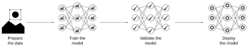
Object detection pipeline
Prepare the data
The first step to train a great model is to have good quality data. When developing this project, I did not find a suitable (and small enough) object detection dataset, so I decided to create my own.
I looked around and saw a Kangaroo sign that I have in my bedroom — a souvenir that I bought to remember my Aussie days. So I decided to build a Kangaroo detector.
To build my dataset, I downloaded 350 kangaroo images from an image search for kangaroos and labeled all of them by hand using the LabelImg application. As we can have more than one animal per image, the process resulted in 520 labeled kangaroos.

Labelling example
In that case, I chose just one class, but the software can be used to annotate multiple classes as well. It’s going to generate an XML file per image (Pascal VOC format) that contains all annotations and bounding boxes.
<annotation>
    <folder>images</folder>
    <filename>kangaroo-0.jpg</filename>
    <path>/home/hugo/Documents/projects/tfjs/dataset/images/kangaroo-0.jpg</path>
  <source>
    <database>Unknown</database>
  </source>
  <size>
    <width>3872</width>
    <height>2592</height>
    <depth>3</depth>
  </size>
  <segmented>0</segmented>
  <object>
    <name>kangaroo</name>
    <pose>Unspecified</pose>
    <truncated>0</truncated>
    <difficult>0</difficult>
    <bndbox>
      <xmin>60</xmin>
      <ymin>367</ymin>
      <xmax>2872</xmax>
      <ymax>2399</ymax>
    </bndbox>
  </object>
</annotation>
XML Annotation example
To facilitate the conversion to TF.record format (below), I then converted the XML of the program above into two CSV files containing the data already split in train and test (80%-20%). These files have 9 columns:
- filename: Image name
- width: Image width
- height: Image height
- class: Image class (kangaroo)
- xmin: Minimum bounding box x coordinate value
- ymin: Minimum bounding box y coordinate value
- xmax: Maximum value of the x coordinate of the bounding box
- ymax: Maximum value of the y coordinate of the bounding box
- source: Image source
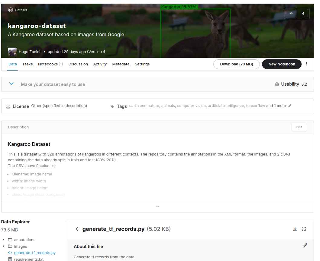
Using LabelImg makes it easy to create your own dataset, but feel free to use my kangaroo dataset, I’ve uploaded it on Kaggle:
Training the model
With a good dataset, it’s time to think about the model.TensorFlow 2 provides an Object Detection API that makes it easy to construct, train, and deploy object detection models. In this project, we’re going to use this API and train the model using a Google Colaboratory Notebook. The remainder of this section explains how to set up the environment, the model selection, and training. If you want to jump straight to the Colab Notebook, click here.
Setting up the environment
Create a new Google Colab notebook and select a GPU as hardware accelerator:
Runtime > Change runtime type > Hardware accelerator: GPU
Clone, install, and test the TensorFlow Object Detection API:
Getting and processing the data
As mentioned before, the model is going to be trained using the Kangaroo dataset on Kaggle. If you want to use it as well, it’s necessary to create a user, go into the account section of Kaggle, and get an API Token:
Getting an API Token
Then, you’re ready to download the data:
Now, it’s necessary to create a labelmap file to define the classes that are going to be used. Kangaroo is the only one, so right-click in the File section on Google Colab and create a New file named labelmap.pbtxt as follows:
 item {
    name: "kangaroo"
    id: 1
}
The last step is to convert the data into a sequence of binary records so that they can be fed into Tensorflow’s object detection API. To do so, transform the data into the TFRecord format using the generate_tf_records.py script available in the Kangaroo Dataset:
Choosing the model
We’re ready to choose the model that’s going to be the Kangaroo Detector. TensorFlow 2 provides 40 pre-trained detection models on the COCO 2017 Dataset. This collection is the TensorFlow 2 Detection Model Zoo and can be accessed here.
Every model has a Speed, Mean Average Precision(mAP) and Output. Generally, a higher mAP implies a lower speed, but as this project is based on a one-class object detection problem, the faster model (SSD MobileNet v2 320×320) should be enough.
Besides the Model Zoo, TensorFlow provides a Models Configs Repository as well. There, it’s possible to get the configuration file that has to be modified before the training. Let’s download the files:
Configure training
As mentioned before, the downloaded weights were pre-trained on the COCO 2017 Dataset, but the focus here is to train the model to recognize one class so these weights are going to be used only to initialize the network — this technique is known as transfer learning, and it’s commonly used to speed up the learning process.
From now, what has to be done is to set up the mobilenet_v2.config file, and start the training. I highly recommend reading the MobileNetV2 paper (Sandler, Mark, et al. – 2018) to get the gist of the architecture.
Choosing the best hyperparameters is a task that requires some experimentation. As the resources are limited in the Google Colab, I am going to use the same batch size as the paper, set a number of steps to get a reasonably low loss, and leave all the other values as default. If you want to try something more sophisticated to find the hyperparameters, I recommend Keras Tuner – an easy-to-use framework that applies Bayesian Optimization, Hyperband, and Random Search algorithms.
With the parameters set, start the training:
To identify how well the training is going, we use the loss value. Loss is a number indicating how bad the model’s prediction was on the training samples. If the model’s prediction is perfect, the loss is zero; otherwise, the loss is greater. The goal of training a model is to find a set of weights and biases that have low loss, on average, across all examples (Descending into ML: Training and Loss | Machine Learning Crash Course).
From the logs, it’s possible to see a downward trend in the values so we say that “The model is converging”. In the next section, we’re going to plot these values for all training steps and the trend will be even clearer.
The model took around 4h to train (with Colab GPU), but by setting different parameters, you can make the process faster or slower. Everything depends on the number of classes you are using and your Precision/Recall target. A highly accurate network that recognizes multiple classes will take more steps and require more detailed parameters tuning.
Validate the model
Now let’s evaluate the trained model using the test data:
The evaluation was done in 89 images and provides three metrics based on the COCO detection evaluation metrics: Precision, Recall and Loss.
The Recall measures how good the model is at hitting the positive class, That is, from the positive samples, how many did the algorithm get right?

Recall
Precision defines how much you can rely on the positive class prediction: From the samples that the model said were positive, how many actually are?

Precision
Setting a practical example: Imagine we have an image containing 10 kangaroos, our model returned 5 detections, being 3 real kangaroos (TP = 3, FN =7) and 2 wrong detections (FP = 2). In that case, we have a 30% recall (the model detected 3 out of 10 kangaroos in the image) and a 60% precision (from the 5 detections, 3 were correct).
The precision and recall were divided by Intersection over Union (IoU) thresholds. The IoU is defined as the area of the intersection divided by the area of the union of a predicted bounding box (B) to a ground-truth box (B)(Zeng, N. – 2018):

Intersection over Union
For simplicity, it’s possible to consider that the IoU thresholds are used to determine whether a detection is a true positive(TP), a false positive(FP) or a false negative (FN). See an example below:

IoU threshold examples
With these concepts in mind, we can analyze some of the metrics we got from the evaluation. From the TensorFlow 2 Detection Model Zoo, the SSD MobileNet v2 320×320 has an mAP of 0.202. Our model presented the following average precisions (AP) for different IoUs:
AP@[IoU=0.50:0.95 | area=all | maxDets=100] = 0.222
AP@[IoU=0.50      | area=all | maxDets=100] = 0.405
AP@[IoU=0.75      | area=all | maxDets=100] = 0.221
That’s pretty good! And we can compare the obtained APs with the SSD MobileNet v2 320×320 mAP as from the COCO Dataset documentation:
We make no distinction between AP and mAP (and likewise AR and mAR) and assume the difference is clear from context.
The Average Recall(AR) was split by the max number of detection per image (1, 10, 100). When we have just one kangaroo per image, the recall is around 30% while when we have up to 100 kangaroos it is around 51%. These values are not that good but are reasonable for the kind of problem we’re trying to solve.
(AR)@[ IoU=0.50:0.95 | area=all | maxDets=  1] = 0.293
(AR)@[ IoU=0.50:0.95 | area=all | maxDets= 10] = 0.414
(AR)@[ IoU=0.50:0.95 | area=all | maxDets=100] = 0.514
The Loss analysis is very straightforward, we’ve got 4 values:
INFO:tensorflow: + Loss/localization_loss: 0.345804
INFO:tensorflow: + Loss/classification_loss: 1.496982
INFO:tensorflow: + Loss/regularization_loss: 0.130125
INFO:tensorflow: + Loss/total_loss: 1.972911
The localization loss computes the difference between the predicted bounding boxes and the labeled ones. The classification loss indicates whether the bounding box class matches with the predicted class. The regularization loss is generated by the network’s regularization function and helps to drive the optimization algorithm in the right direction. The last term is the total loss and is the sum of three previous ones.
Tensorflow provides a tool to visualize all these metrics in an easy way. It’s called TensorBoard and can be initialized by the following command:
%load_ext tensorboard
%tensorboard --logdir '/content/training/'
This is going to be shown, and you can explore all training and evaluation metrics.

Tensorboard — Loss
In the tab IMAGES, it’s possible to find some comparisons between the predictions and the ground truth side by side. A very interesting resource to explore during the validation process as well.

Tensorboard — Testing images
Exporting the model
Now that the training is validated, it’s time to export the model. We’re going to convert the training checkpoints to a protobuf (pb) file. This file is going to have the graph definition and the weights of the model.
As we’re going to deploy the model using TensorFlow.js and Google Colab has a maximum lifetime limit of 12 hours, let’s download the trained weights and save them locally. When running the command files.download(‘/content/saved_model.zip”), the colab will prompt the file automatically.
If you want to check if the model was saved properly, load, and test it. I’ve created some functions to make this process easier so feel free to clone the inferenceutils.py file from my GitHub to test some images.
Everything is working well, so we’re ready to put the model in production.
Deploying the model
The model is going to be deployed in a way that anyone can open a PC or mobile camera and perform inferences in real-time through a web browser. To do that, we’re going to convert the saved model to the Tensorflow.js layers format, load the model in a javascript application and make everything available on Glitch.
Converting the model
At this point, you should have something similar to this structure saved locally:
├── inference-graph
│ ├── saved_model
│ │ ├── assets
│ │ ├── saved_model.pb
│ │ ├── variables
│ │ ├── variables.data-00000-of-00001
│ │ └── variables.index
Before we start, let’s create an isolated Python environment to work in an empty workspace and avoid any library conflict. Install virtualenv and then open a terminal in the inference-graph folder and create and activate a new virtual environment:
virtualenv -p python3 venv
source venv/bin/activate
Install the TensorFlow.js converter:
pip install tensorflowjs[wizard]
Start the conversion wizard:
tensorflowjs_wizard
Now, the tool will guide you through the conversion, providing explanations for each choice you need to make. The image below shows all the choices that were made to convert the model. Most of them are the standard ones, but options like the shard sizes and compression can be changed according to your needs.
To enable the browser to cache the weights automatically, it’s recommended to split them into shard files of around 4MB. To guarantee that the conversion is going to work, don’t skip the op validation as well, not all TensorFlow operations are supported so some models can be incompatible with TensorFlow.js — See this list for which ops are currently supported.

Model conversion using Tensorflow.js Converter (Full resolution image here
If everything worked well, you’re going to have the model converted to the Tensorflow.js layers format in the web_modeldirectory. The folder contains a model.json file and a set of sharded weights files in a binary format. The model.json has both the model topology (aka “architecture” or “graph”: a description of the layers and how they are connected) and a manifest of the weight files (Lin, Tsung-Yi, et al).
└ web_model
  ├── group1-shard1of5.bin
  ├── group1-shard2of5.bin
  ├── group1-shard3of5.bin
  ├── group1-shard4of5.bin
  ├── group1-shard5of5.bin
  └── model.json
Configuring the application
The model is ready to be loaded in javascript. I’ve created an application to perform inferences directly from the browser. Let’s clone the repository to figure out how to use the converted model in real-time. This is the project structure:
├── models
│   └── kangaroo-detector
│       ├── group1-shard1of5.bin
│       ├── group1-shard2of5.bin
│       ├── group1-shard3of5.bin
│       ├── group1-shard4of5.bin
│       ├── group1-shard5of5.bin
│       └── model.json
├── package.json
├── package-lock.json
├── public
│   └── index.html
├── README.MD
└── src
    ├── index.js
    └── styles.css
For the sake of simplicity, I already provide a converted kangaroo-detector model in the models folder. However, let’s put the web_model generated in the previous section in the models folder and test it.
The first thing to do is to define how the model is going to be loaded in the function load_model (lines 10–15 in the file src>index.js). There are two choices.
The first option is to create an HTTP server locally that will make the model available in a URL allowing requests and be treated as a REST API. When loading the model, TensorFlow.js will do the following requests:
GET /model.json
GET /group1-shard1of5.bin
GET /group1-shard2of5.bin
GET /group1-shard3of5.bin
GET /group1-shardo4f5.bin
GET /group1-shardo5f5.bin
If you choose this option, define the load_model function as follows:
  async function load_model() {
    // It's possible to load the model locally or from a repo
    // You can choose whatever IP and PORT you want in the "http://127.0.0.1:8080/model.json"     just set it before in your https server
    const model = await loadGraphModel("http://127.0.0.1:8080/model.json");
    //const model = await loadGraphModel("https://raw.githubusercontent.com/hugozanini/TFJS-object-detection/master/models/web_model/model.json");
    return model;
}
Then install the http-server:
npm install http-server -g
Go to models > web_model and run the command below to make the model available at http://127.0.0.1:8080 . This a good choice when you want to keep the model weights in a safe place and control who can request inferences to it. The -c1 parameter is added to disable caching, and the –cors flag enables cross origin resource sharing allowing the hosted files to be used by the client side JavaScript for a given domain.
http-server -c1 --cors .
Alternatively you can upload the model files somewhere, in my case, I chose my own Github repo and referenced to the model.json URL in the load_model function:
async function load_model() {
    // It's possible to load the model locally or from a repo
    //const model = await loadGraphModel("http://127.0.0.1:8080/model.json");
    const model = await loadGraphModel("https://raw.githubusercontent.com/hugozanini/TFJS-object-detection/master/models/web_model/model.json");
    return model;
}
This is a good option because it gives more flexibility to the application and makes it easier to run on some platform as Glitch.
Running locally
To run the app locally, install the required packages:
npm install
And start:
npm start
The application is going to run at http://localhost:3000 and you should see something similar to this:

Application running locally
The model takes from 1 to 2 seconds to load and, after that, you can show kangaroos images to the camera and the application is going to draw bounding boxes around them.
Publishing in Glitch
Glitch is a simple tool for creating web apps where we can upload the code and make the application available for everyone on the web. Uploading the model files in a GitHub repo and referencing to them in the load_model function, we can simply log into Glitch, click on New project > Import from Github and select the app repository.
Wait some minutes to install the packages and your app will be available in a public URL. Click on Show > In a new window and a tab will be open. Copy this URL and past it in any web browser (PC or Mobile) and your object detection will be ready to run. See some examples in the video below:
Running the model on different devices
First, I did a test showing a kangaroo sign to verify the robustness of the application. It showed that the model is focusing specifically on the kangaroo features and did not specialize in irrelevant characteristics that were present in many images, such as pale colors or shrubs.
Then, I opened the app on my mobile and showed some images from the test set. The model runs smoothly and identifies most of the kangaroos. If you want to test my live app, it is available here (glitch takes some minutes to wake up).
Besides the accuracy, an interesting part of these experiments is the inference time — everything runs in real-time in the browser via JavaScript. Good object detection models running in the browser and using few computational resources is a must in many applications, mostly in industry. Putting the Machine Learning model on the client-side means cost reduction and safer applications as user privacy is preserved as there is no need to send the information to any server to perform the inference.
Next steps
Object detection in the browser can solve a lot of real-world problems and I hope this article will serve as a basis for new projects involving Computer Vision, Python, TensorFlow and Javascript.
As the next steps, I’d like to make more detailed training experiments. Due to the lack of resources, I could not try many different parameters and I’m sure that there is a lot of room for improvements in the model.
I’m more focused on the models’ training, but I’d like to see a better user interface for the app. If someone is interested in contributing to the project, feel free to create a pull request in the project repo. It will be nice to make a more user-friendly application.
If you have any questions or suggestions you can reach me out on Linkedin. Thanks for reading!


 Pradeep Singh is a Solutions Architect at Amazon Web Services. He helps AWS customers take advantage of AWS services to design scalable and secure applications. His expertise spans Application Architecture, Containers, Analytics and Machine Learning.
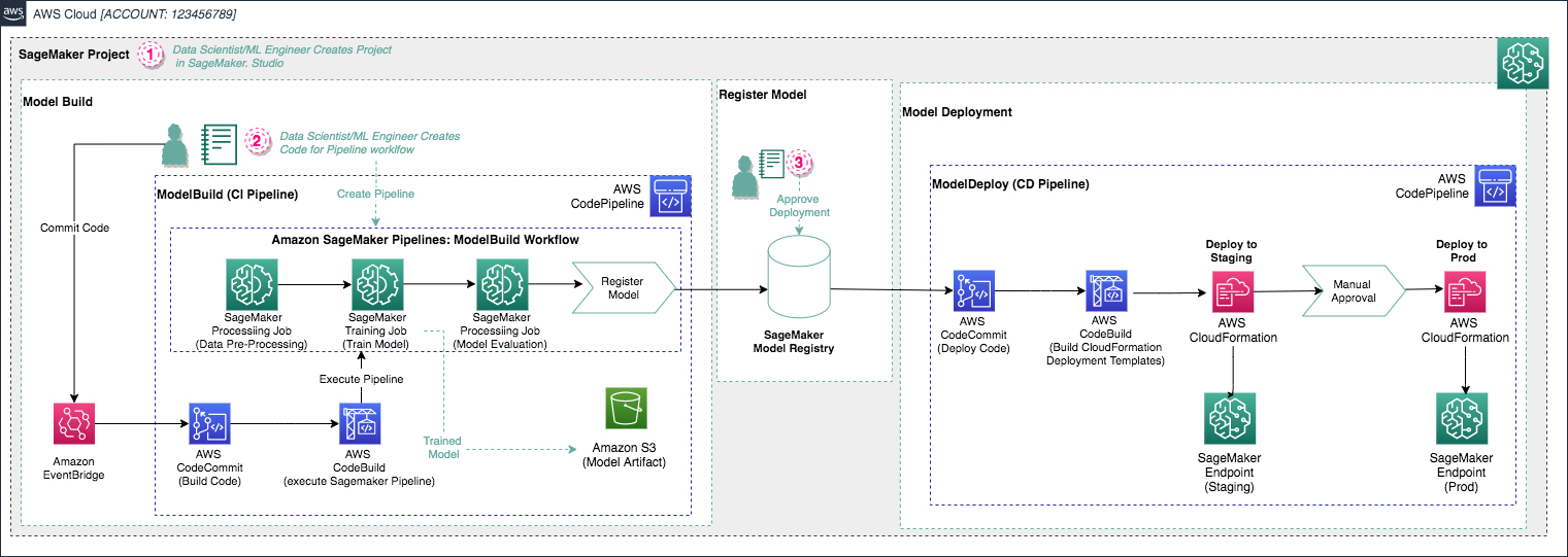

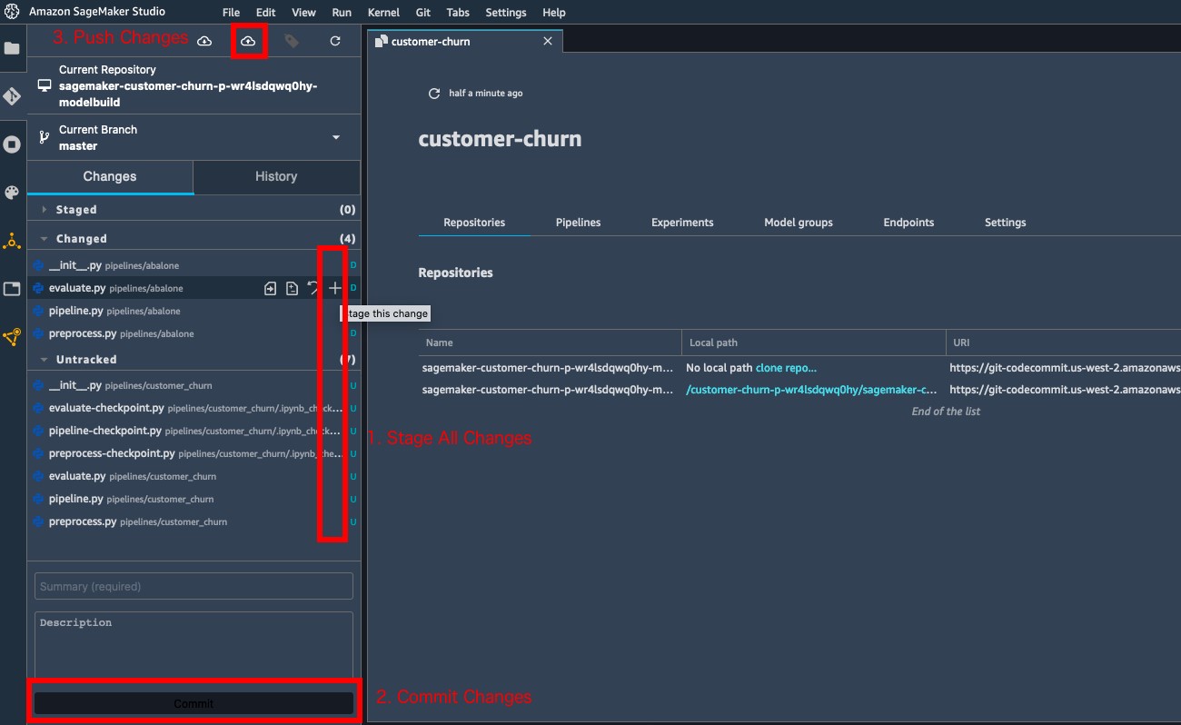 The following screenshot shows our pipeline details.
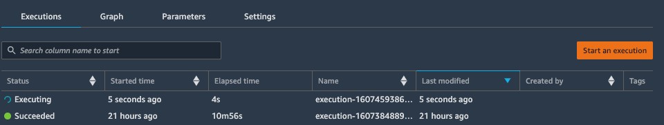 Choosing the pipeline run displays the steps of the pipeline, which you can monitor.
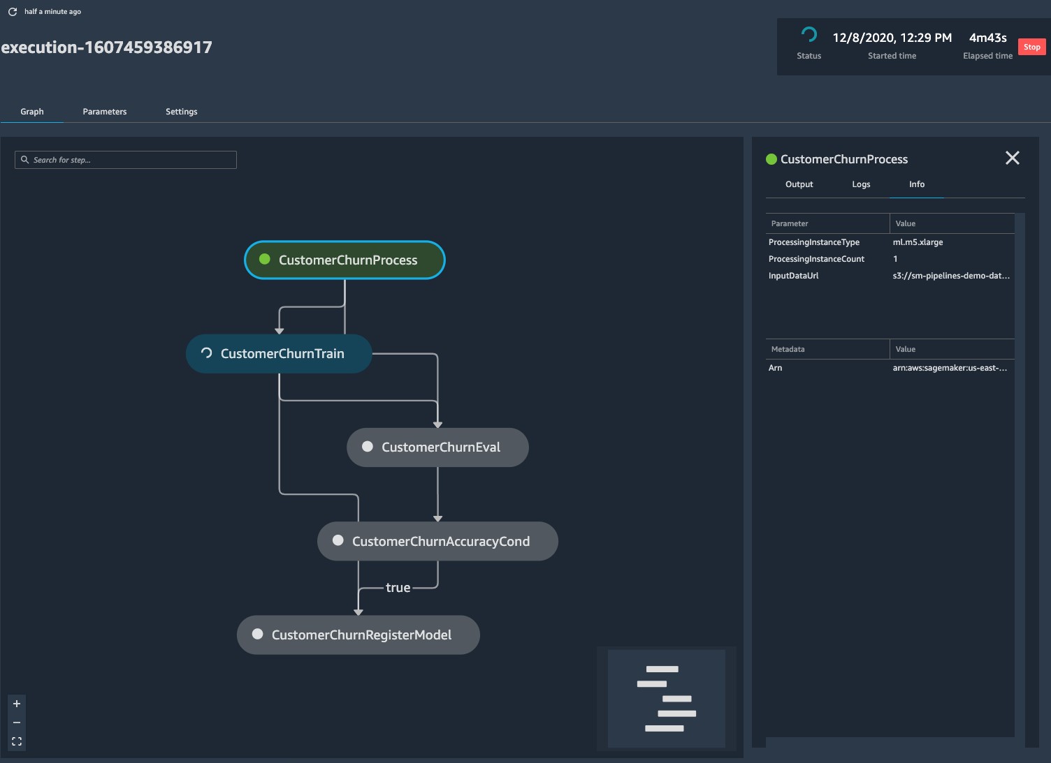

 Sean Morgan is an AI/ML Solutions Architect at AWS. He previously worked in the semiconductor industry, using computer vision to improve product yield. He later transitioned to a DoD research lab where he specialized in adversarial ML defense and network security. In his free time, Sean is an active open-source contributor and maintainer, and is the special interest group lead for TensorFlow Addons.
 Hallie Weishahn is an AI/ML Specialist Solutions Architect at AWS, focused on leading global standards for MLOps. She previously worked as an ML Specialist at Google Cloud Platform. She works with product, engineering, and key customers to build repeatable architectures and drive product roadmaps. She provides guidance and hands-on work to advance and scale machine learning use cases and technologies. Troubleshooting top issues and evaluating existing architectures to enable integrations from PoC to a full deployment is her strong suit.
 Shelbee Eigenbrode is an AI/ML Specialist Solutions Architect at AWS. Her current areas of depth include DevOps combined with ML/AI. She has been in technology for 23 years, spanning multiple roles and technologies. With over 35 patents granted across various technology domains, her passion for continuous innovation combined with a love of all things data turned her focus to the field of d ata science. Combining her backgrounds in data, DevOps, and machine learning, her current passion is helping customers to not only embrace data science but also ensure all models have a path to production by adopting MLOps practices. In her spare time, she enjoys reading and spending time with family, including her fur family (aka dogs), as well as friends.


 As a Principal Prototyping Engagement Manager, Dr. Markus Bestehorn is responsible for building business-critical prototypes with AWS customers, and is a specialist for IoT and machine learning. His “career” started as a 7-year-old when he got his hands on a computer with two 5.25” floppy disks, no hard disk, and no mouse, on which he started writing BASIC, and later C as well as C++ programs. He holds a PhD in computer science and all currently available AWS certifications. When he’s not on the computer, he runs or climbs mountains.