Center to support novel approaches to trust-centric machine learning and AI innovation.Read More
New Games, New Features — That’s GFN Thursday
We love PC games. The newest titles and the greatest classics. FPS, RPG, grand strategy, squad-based tactics, single-player, multiplayer, MMO — you name it, we love it.
There are more than 800 games on GeForce NOW — including 80 of the biggest free-to-play games — streaming straight from the cloud. And thanks to the explosive growth of PC gaming in recent years, there are more games to play than ever.
Fun fact: those games often launch on Thursdays, right alongside our client and backend updates. That makes Thursday our favorite day of the week. So let’s formalize it, right?
This is GFN Thursday — our weekly celebration of the newest games, features and news, streaming from the cloud to you.
This week’s a doozy, too. But before we get into the games, let’s set the stage and answer a few questions.
What is GFN Thursday?
GFN Thursday is our ongoing commitment to bringing great PC games and service updates to our members each week. Come back every Thursday to discover what’s new in the cloud, including games, exclusive features, and news on GeForce NOW.
Why Thursdays?
Because Mondays are boring? Seriously, over the course of the past year, many of our most played games either launched or released major season updates on Thursdays — and we aim to support these launches as soon after their release as possible.
Many of the top free-to-play games, from Fortnite to Apex Legends, Destiny 2 and more, also release major season updates for Thursdays. We’re committed to supporting each new content release the moment it’s available, with updates rolling out to members across all our data centers, in all of our regions as quickly as possible.
Our members love to learn what’s coming each week to the GeForce NOW library and plan their gaming for the weekend. We do, too. With GFN Thursday updates every week, you’ll always know what’s ready to play across your devices, even if you’re away from your gaming rig.
What if I want to know what games are coming in the future?
Okay, then the first GFN Thursday of each month is for you. That’s when we’ll share the games we anticipate adding to GeForce NOW throughout that month.
This list may not be every game that releases in a month, however. Things move fast, and we know there will be surprises. In January alone, we shared 23 games coming to GeForce NOW, with HITMAN 3 and Everspace 2 being late-breaking additions we were also able to welcome this month.
Games will continue to be added every week, but that first GFN Thursday of the month will give you a glimpse at what to expect. That way you can shop with confidence, knowing what’s to come.
Okay, so what’s happening this GFN Thursday?
Finally, let’s get to the good stuff. The complete list of games joining GeForce NOW this week can be found below, but here are a few highlights:
The Medium (Steam & Epic Games Store)
Founders can play with RTX ON and discover a dark mystery only a medium can solve. Travel to an abandoned communist resort and use your psychic abilities to uncover its deeply disturbing secrets, solve dual-reality puzzles, survive encounters with sinister spirits and explore two realities at the same time.
Immortals Fenyx Rising Demo (Ubisoft Connect & Epic Games Store)
In this free demo from Ubisoft, play as Fenyx, a new winged demigod, on a quest to save the Greek gods and their home from a dark curse. Take on mythological beasts, master the legendary powers of the gods and defeat Typhon, the deadliest Titan in Greek mythology, in an epic fight for the ages.
Members with the full game and Season Pass can also play the new Immortals Fenyx Rising DLC, A New God, on Jan. 28.
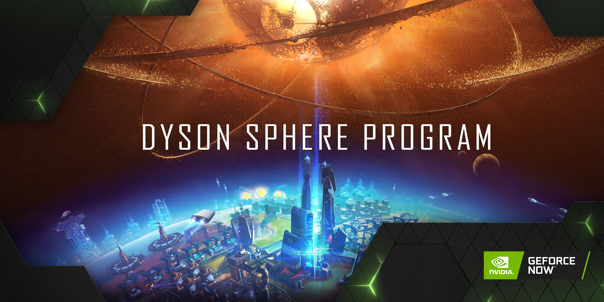
Dyson Sphere Program (Steam)
Build the most efficient intergalactic factory in this space simulation strategy game. Harness the power of stars, collect resources, plan and design production lines and develop your interstellar factory from a small space workshop to a galaxy-wide industrial empire.


Here’s the full list for Jan. 28. What are you looking forward to playing? Let us know below.
We’ll see you next week for a very exciting one-year anniversary edition of GFN Thursday!
- The Medium (Steam, Epic Games Store)
- Immortals Fenyx Rising Demo (Ubisoft Connect, Epic Games Store)
- Beholder (Steam)
- Caves of Qud (Steam)
- Dyson Sphere Program (Steam)
- Kathy Rain (Steam)
- Neon Abyss (Epic Games Store)
- Gods Will Fall (launching Friday on Steam, Epic Games Store)
The post New Games, New Features — That’s GFN Thursday appeared first on The Official NVIDIA Blog.
Deepset achieves a 3.9x speedup and 12.8x cost reduction for training NLP models by working with AWS and NVIDIA
This is a guest post from deepset (creators of the open source frameworks FARM and Haystack), and was contributed to by authors from NVIDIA and AWS.
At deepset, we’re building the next-level search engine for business documents. Our core product, Haystack, is an open-source framework that enables developers to utilize the latest NLP models for semantic search and question answering at scale. Our software as a service (SaaS) platform, Haystack Hub, is used by developers from various industries, including finance, legal, and automotive, to find answers in all kinds of text documents. You can use these answers to improve the search experience, cover the long-tail of chat bot queries, extract structured data from documents, or automate invoicing processes.
Pretrained language models like BERT, RoBERTa, and ELECTRA form the core for this latest type of semantic search and many other NLP applications. Although plenty of English models are available, the availability for other languages and more industry-specific terms (such as finance or automotive) is usually very limited and often complicates applications in the industry. Therefore, we regularly train language models for languages not covered by existing models (such as German BERT and German ELECTRA), models for special domains (such as finance and aerospace), or even models for client-specific jargon.
Challenge
Pretraining language models from scratch typically involves two major challenges: cost and development effort.
Training a language model is an extremely compute-intensive task and requires multiple GPUs running for multiple days. To give you a rough idea, training the original RoBERTa model took about 1 day on 1024 NVIDIA V100 GPUs.
Computation costs aren’t the only thing that can stress your budget. A considerable amount of manual development is required to create the training data and vocabulary, configure hyperparameters, start and monitor training jobs, and run periodical evaluation of different model checkpoints. In our first training runs, we also found several bugs only after multiple hours of training, resulting in a slow development cycle. In summary, language model training can be a painful job for a developer and easily consumes multiple days of work.
Solution
In a collaborative effort, AWS, NVIDIA, and deepset were able to complete training 3.9 times faster while lowering cost by 12.8 times and reducing developer effort from days to hours. We optimized the GPU utilization during training via PyTorch’s DistributedDataParallel (DDP) and enabled larger batch sizes by switching to Automatic Mixed Precision (AMP). Furthermore, we introduced a StreamingDataSilo that allows us to load the training data lazily from disk and to do the preprocessing on the fly, leading to a lower memory footprint and no initial preprocessing time. Last but not least, we integrated the training with Amazon SageMaker to reduce manual development effort and benefit from around a 70% cost reduction by using Amazon Elastic Compute Cloud (Amazon EC2) Spot Instances.
In this post, we explore each of these technologies and their impact on improving BERT training performance.
DistributedDataParallel
DistributedDataParallel (DDP) implements distributed data parallelism in PyTorch. This is a key module that’s essential for running training jobs at scale, on multiple machines or on multiple GPUs in a single machine. DDP parallelizes a given network module by splitting the input across specified devices (GPUs). The input is split in the batch dimension. The network module is replicated on each device, and each such replica handles a slice of the input. The gradients from each device are averaged during a backward pass. DDP is used in conjunction with the torch.distributed framework, which handles all communication and synchronization in distributed training jobs with PyTorch.
Before DDP was introduced, torch.nn.DataParallel (DP) was the standard module for doing single-machine multi-GPU training in PyTorch. The system in DP works as follows:
- The entire batch of input is loaded on the main thread.
- The batch is split and scattered across all the GPUs in the network.
- Each GPU runs the forward pass on its batch, split on a separate thread.
- The network outputs are gathered on the master GPU, the loss value is computed, and this loss value is then scattered across the other GPUs.
- Each GPU uses the loss value to run a backward pass and compute the gradients.
- The gradients are reduced on the master GPU and the model parameters on the master GPU are updated. This completes one iteration of training.
- To ensure all GPUs have the latest model parameters, they are broadcasted to the other GPUs at the start of the next iteration.
This design of DP has several inefficiencies:
- Uneven GPU utilization – Only the primary GPU handles loss calculation, gradient reduction, and parameter updates, which leads to higher GPU memory consumption compared to the rest of the GPUs
- Unnecessary broadcast at the beginning of each iteration – Because the model parameters are only updated in the master GPU, they need to be broadcast to the other GPUs before every iteration
- Unnecessary gathering step – There is an unnecessary gathering step of model outputs on the GPU
- Redundant data copies – Data is first copied to the master GPU, which is then split and copied over to the other GPUs
- Multithreading overhead – Performance overhead caused by the Global Interpreter Lock (GIL) of the Python interpreter
DDP eliminates all such inefficiencies of DP. DDP uses a multiprocessing architecture, unlike the multithreaded one in DP. This means each GPU has its own dedicated process which runs independently and there is no master GPU anymore. Each process starts by loading its own split of data from the disk. Then the forward pass and loss computation is run independently on each GPU. This eliminates the need for gathering network outputs. During the backward pass, the gradients are AllReduced across the GPUs. Averaging the gradients with AllReduce ensures that the gradients in each GPU are identical. As a result, the model updates in each GPU are identical as well, which eliminates the need for parameter broadcast at the start of the next iteration.
Results with DDP
With DP, the GPU memory utilization was skewed towards the master GPU, which consumed 15 GB, whereas all other GPUs consumed 6 GB. With DDP, the memory consumption was split equally across 4 GPUs, or about 9 GB on each. This also allowed us to increase the per GPU batch size, which further contributed to the speedup in throughput. We reduced the number of gradient accumulation steps to keep the effective batch size constant, to ensure that there was no impact in convergence.
The following table shows the results on a P3.8xlarge instance with 4 NVIDIA V100 GPUs. With DDP, the training time reduced from 616 hours to 347 hours.
| Run | Batch Size | Accumulation Steps | Effective Batch Size | Throughput (Effective Batches per Hour) | Total Estimated Training Time (Hours) |
| BERT Training with DP | 105 | 9 | 945 | 811 | 616 |
| BERT Training with DDP | 240 | 4 | 960 | 1415 | 347 |
The following screenshots show the GPU performance profiles captured by the NVIDIA Nsight Systems. The first screenshot shows the profile while running with DP. Light blue bars in the box marked as “GPU Utilization” show if GPUs are busy. Gaps between the blue areas show that the GPU utilization is zero. The red blocks in between are CPU to GPU memory copy operations. An additional blue block is between the memory copies, which is the aggregation operation that is computed on a single GPU.
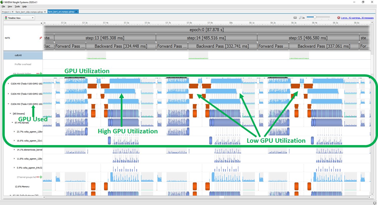
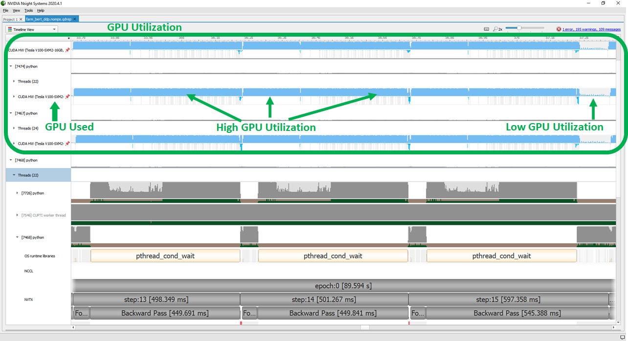
The following screenshot shows high GPU utilization with DDP, which effectively deprecates all those inefficiencies.
Training with Automatic Mixed Precision
Automatic Mixed Precision (AMP) speeds up deep learning training with minimal impact to final accuracy. Traditionally, 32-bit precision floating point (FP32) variables are commonly used in deep learning training. You can improve speed of training with 16-bit precision floating point (FP16) variables because it requires lower storage and less memory bandwidth. However, training with lower precision could decrease the accuracy of the results. Mixed precision training is a balanced approach to achieve the computational speed up of lower precision training while maintaining accuracy close to FP32 precision training. Training with mixed precision provides additional speedup by using NVIDIA Tensor Cores, which are specialized hardware available on NVIDIA GPUs for accelerated computation.
To maintain accuracy, training with mixed precision involves the following steps:
- Port the model to use the FP16 datatype where appropriate.
- Handle specific functions or operations that must be done in FP32 to maintain accuracy.
- Add loss scaling to preserve small gradient values.
The AMP feature handles all these steps for deep learning training. As of this writing, all popular deep learning frameworks like PyTorch, TensorFlow, and Apache MXNet support AMP.
AMP in PyTorch was supported via the NVIDIA APEX library. AMP support has recently been moved to PyTorch core with the 1.6 release.
AMP in APEX library provides four levels of optimization for different application usage. Optimization levels O1 and O2 are both mixed precision modes with slight differences, where O1 is the recommended way for typical use cases and 02 is more aggressively converting most layers into FP16 mode. O0 and O4 opt levels are actually the FP32 mode and FP16 mode designed for reference only.
The following table shows the impact of applying AMP along with DDP. Without AMP, batch size up to 240 could be run on the GPU. With AMP, the larger batch size of 320 could be supported, reducing the total training time from 347 hours to 223 hours
| Run | Batch Size | Accumulation Steps | Effective Batch Size | Throughput (Effective Batches per Hour) | Total Estimated Training Time (Hours) |
| BERT Training with DDP | 240 | 4 | 960 | 1415 | 347 |
| BERT Training with DDP & AMP 01 | 304 | 3 | 912 | 2025 | 243 |
| BERT Training with DDP & AMP 02 | 320 | 3 | 960 | 2210 | 223 |
As mentioned earlier, AMP O2 converts more layers into FP16 mode, so we can run DDP and AMP O2 with a larger batch size and get a better throughput compared to DDP and AMP O1. When selecting between these two opt levels, you should do a validation of the prediction results to make sure AMP O2 meets your accuracy requirements.
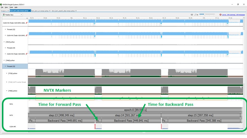
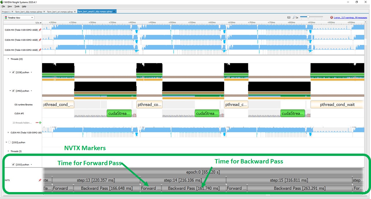
The following screenshot shows the GPU performance profile after applying DDP but running the deep learning training with FP32 variables. In this profile, we have added custom markers called NVTX markers, which show the time taken for each epoch, each step, and the time for the forward and backward pass.
The following screenshot shows the profile after enabling AMP with opt level O2. The time to run a forward and backward pass reduced significantly even though we increased the batch size for training when using AMP.
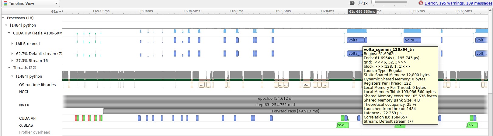
Earlier, we mentioned that AMP utilizes Tensor Cores available on NVIDIA GPU hardware for significant speedup for deep learning training. GPU performance profiles show when operations are utilizing Tensor Cores. The following screenshot shows a sample GPU kernel that is run in FP32 mode. The GPU operation is marked here as the volta_sgemm kernel.
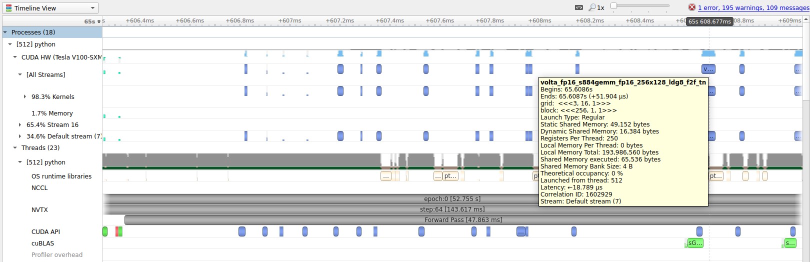
The following screenshot shows similar operations run in FP16 mode, which utilizes Tensor Cores. Kernels running with Tensor Cores are marked as volta_fp16_s884gemm.
Data pipeline
The datasets used for training language models typically contain 10–200 GB of raw text data. Loading the whole dataset in RAM can be challenging. Furthermore, the typical pipeline of first running the preprocessing for all data and then pulling batches during training isn’t optimal because the up-front preprocessing can take multiple hours in which we don’t utilize the GPUs on the server.
Therefore, we introduced a StreamingDataSilo, which loads data lazily from disk just in time when it’s needed in the training loop. The whole preprocessing happens on the fly. Our implementation builds upon PyTorch’s IterableDataset and DistributedSampler, but requires some custom parts to ensure enough preprocessed batches are always in the queue for our trainer, so that the GPU never has to wait for the next batch to be ready. For implementation steps, see the GitHub repo. Together with an increased number of workers to fill the queue, we ended up with another 28% throughput improvement, as shown in the following table.
| Run | Batch Size | Accumulation Steps | Effective Batch Size | Throughput (Effective Batches per Hour) | Total Estimated Training Time (Hours) |
| DDP with 8 workers | 320 | 3 | 960 | 2210 | 223 |
| DDP with 16 workers | 320 | 3 | 960 | 3077 | 160 |
A second tricky case that we had to handle was related to the unknown number of batches in our dataset and the distributed training via DDP. If the batches in your dataset can’t be evenly distributed across the number of workers, some workers don’t get any batches in the last step of the epoch while others do. This asynchronicity can crash your whole training run or result in a deadlock (for a related PyTorch issue, see [RFC] Join-based API to support uneven inputs in DDP). We handled this by adding a small synchronization step where all workers communicate if they still have data left. For implementation details, see the GitHub repo.
Spot Instances
Besides reducing the total training time, using EC2 Spot Instances is another compelling approach to reduce training costs. This is pretty straightforward to configure in SageMaker; just set the parameter EnableManagedSpotTraining to True when launching your training job. SageMaker launches your training job and saves checkpoints periodically. When your Spot Instance ends, SageMaker takes care of spinning up a new instance and loading the latest checkpoint to continue training from there.
In your code, you need to make sure to save regular checkpoints containing the states of all the objects that are relevant for your training session. This includes not only your model weights, but also the states of your optimizer, the data loader, and all random number generators to replicate the results from your continuous runs without Spot Instances. For implementation details, see the GitHub repo.
In our test runs, we achieved around 70% cost savings in comparison to regular On-Demand Instances.
Conclusion
Language models have become the backbone of modern NLP. Although using existing public models works well in many cases, many domains with special languages can benefit from training a new model from scratch. Having a fast, simple, and cheap training pipeline is essential for these big training jobs. In addition, the increased efficiency of training jobs reduces our energy usage and lowers our carbon footprint. By tackling different areas of FARM’s training pipeline, we were able to significantly optimize the resource utilization. In the end, we were able to achieve a speedup in training time of 3.9 times faster, a 12.8 times reduction in training cost, and reduced the developer effort required from days to hours.
If you’re interested in training your own BERT model, you can look at the open-source code in FARM or try our free SageMaker algorithm on the AWS Marketplace.
About the Authors
Abhinav Sharma is a Software Engineer at AWS Deep Learning. He works on bringing state-of-the-art deep learning research to customers, building products that help customers use deep learning engines. Outside of work, he enjoys playing tennis, noodling on his guitar and watching thriller movies.
Malte Pietsch is Co-Founder & CTO at deepset, where he builds the next-level enterprise search engine fueled by open source and NLP. He holds a M.Sc. with honors from TU Munich and conducted research at Carnegie Mellon University. He is an open-source lover, likes reading papers before breakfast, and is obsessed with automating the boring parts of our work.
Khaled ElGalaind is the engineering manager for AWS Deep Engine Benchmarking, focusing on performance improvements for AWS machine learning customers. Khaled is passionate about democratizing deep learning. Outside of work, he enjoys volunteering with the Boy Scouts, BBQ, and hiking in Yosemite.
Jiahong Liu is a Solution Architect on the NVIDIA Cloud Service Provider team, where he helps customers adopt ML and AI solutions with better utilization of NVIDIA’s GPU to solve their business challenges.
Anish Mohan is a Machine Learning Architect at NVIDIA and the technical lead for ML and DL engagements with key NVIDIA customers in the greater Seattle region. Before NVIDIA, he was at Microsoft’s AI Division, working to develop and deploy AI and ML algorithms and solutions.
NVIDIA Expands vGPU Software to Accelerate Workstations, AI Compute Workloads
Designers, engineers, researchers, creative professionals all need the flexibility to run complex workflows – no matter where they’re working from.
With the newest release of NVIDIA virtual GPU (vGPU) technology, enterprises can provide their employees with more power and flexibility through GPU-accelerated virtual machines from the data center or cloud.
Available now, the latest version of our vGPU software brings GPU virtualization to a broad range of workloads — such as virtual desktop infrastructure, high-performance graphics, data analytics and AI — thanks to its support for the new NVIDIA A40 and NVIDIA A100 80GB GPUs. The new release also supports the NVIDIA GPU Operator, a software framework that simplifies GPU deployment and management.
Powerful Performance for Power Users
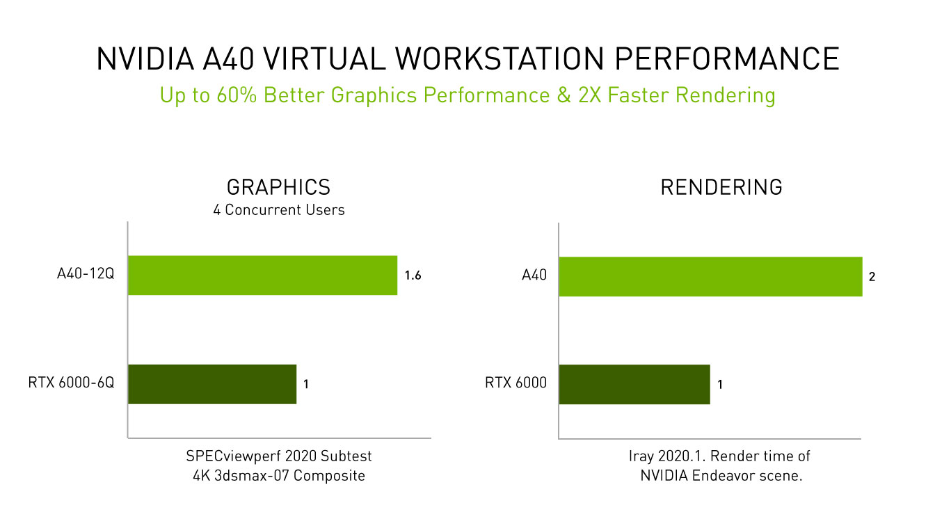
NVIDIA RTX Virtual Workstation (vWS) software is a major component of the vGPU portfolio, designed to help users run graphics-intensive applications on virtual workstations. With NVIDIA A40 powering NVIDIA RTX vWS, professionals can achieve up to 60 percent(1) faster virtual workstation performance per user and 2x(2) faster rendering than the previous generation RTX 6000 GPUs.
NVIDIA A40 includes second-generation RT Cores and third-generation Tensor Cores to help users accelerate workloads like photorealistic rendering of movie content, architectural design evaluations, and virtual prototyping of product designs. With 48GB of GPU memory, professionals can easily work with massive datasets and run workloads like data science or simulation with even larger model sizes.
NVIDIA A40 support with the latest vGPU software enables complex graphics workloads to be run in a virtualized environment with performance that is on par with bare metal.
“With support for NVIDIA’s latest vGPU software, and the new NVIDIA A40 with Citrix Hypervisor 8.2 and Citrix Virtual Desktops, we can continue providing the performance customers need to run graphics-intensive visualization applications as their data and workloads grow,” said Calvin Hsu, vice president of product management at Citrix. “The combination of Citrix and NVIDIA virtualization technologies provides access to these applications from anywhere, with an experience that is indistinguishable from a physical workstation.”
The NVIDIA vGPU January 2021 software release supports the NVIDIA A100 80GB to deliver increased memory bandwidth, unlocking more power for large models. This builds on the September release, which introduced compute features that included support for the NVIDIA A100 Tensor Core GPU, the most advanced GPU for AI and high performance computing.
Additional new features include simplified GPU management in Kubernetes through NVIDIA GPU Operator, which is now supported with NVIDIA Virtual Compute Server and NVIDIA RTX vWS software. Containers, including the GPU-optimized software available in the NGC catalog, can be easily deployed and managed in VMs.
With this new release, customers and IT professionals can continue managing their multi-tenant workflows running in virtual machines using popular hypervisors, like Red Hat Enterprise Linux, while the certified GPU Operator brings a similar experience to containerized deployments on top of Red Hat virtualization platforms using Red Hat OpenShift.
“The combination of NVIDIA’s latest generation A40 GPU and NVIDIA vGPU software, supported with Red Hat Enterprise Linux and Red Hat Virtualization, offers a powerful platform capable of serving some of the most demanding workloads ranging from AI/ML to visualization in the oil and gas as well as media and entertainment industries,” said Steve Gordon, director of product management at Red Hat. “As organizations transform and increasingly use containers orchestrated by Kubernetes as key building blocks for their applications, we see Red Hat OpenShift as a likely destination for containerized and virtualized workloads alike.”
To find a certified server, see the NVIDIA vGPU Certified Server page.
Learn more about NVIDIA vGPU software portfolio, which includes:
- NVIDIA RTX Virtual Workstation (RTX vWS) (formerly known as Quadro Virtual Data Center Workstation or Quadro vDWS)
- NVIDIA Virtual Compute Server (vCS)
- NVIDIA Virtual PC (vPC) (formerly known as GRID vPC)
- NVIDIA Virtual Applications (vApps) (formerly known as GRID vApps)
1. Tested on a server with Intel Xeon Gold 6154 3.0GHz 3.7GHz Turbo, RHEL 8.2, vGPU 12.0 software, running four concurrent users per GPU, RTX6000P-6Q versus A40-12Q, running SPECviewperf 2020 Subtest 4K 3dsmax-07 composite.
2. Iray 2020.1. Render time (seconds) of NVIDIA Endeavor scene.
The post NVIDIA Expands vGPU Software to Accelerate Workstations, AI Compute Workloads appeared first on The Official NVIDIA Blog.
Addressing Range Anxiety with Smart Electric Vehicle Routing
Posted by Kostas Kollias and Sreenivas Gollapudi, Research Scientists, Geo Algorithms Team, Google Research
Mapping algorithms used for navigation often rely on Dijkstra’s algorithm, a fundamental textbook solution for finding shortest paths in graphs. Dijkstra’s algorithm is simple and elegant — rather than considering all possible routes (an exponential number) it iteratively improves an initial solution, and works in polynomial time. The original algorithm and practical extensions of it (such as the A* algorithm) are used millions of times per day for routing vehicles on the global road network. However, due to the fact that most vehicles are gas-powered, these algorithms ignore refueling considerations because a) gas stations are usually available everywhere at the cost of a small detour, and b) the time needed to refuel is typically only a few minutes and is negligible compared to the total travel time.
This situation is different for electric vehicles (EVs). First, EV charging stations are not as commonly available as gas stations, which can cause range anxiety, the fear that the car will run out of power before reaching a charging station. This concern is common enough that it is considered one of the barriers to the widespread adoption of EVs. Second, charging an EV’s battery is a more decision-demanding task, because the charging time can be a significant fraction of the total travel time and can vary widely by station, vehicle model, and battery level. In addition, the charging time is non-linear — e.g., it takes longer to charge a battery from 90% to 100% than from 20% to 30%.
 |
| The EV can only travel a distance up to the illustrated range before needing to recharge. Different roads and different stations have different time costs. The goal is to optimize for the total trip time. |
Today, we present a new approach for routing of EVs integrated into the latest release of Google Maps built into your car for participating EVs that reduces range anxiety by integrating recharging stations into the navigational route. Based on the battery level and the destination, Maps will recommend the charging stops and the corresponding charging levels that will minimize the total duration of the trip. To accomplish this we engineered a highly scalable solution for recommending efficient routes through charging stations, which optimizes the sum of the driving time and the charging time together.
 |
| The fastest route from Berlin to Paris for a gas fueled car is shown in the top figure. The middle figure shows the optimal route for a 400 km range EV (travel time indicated – charging time excluded), where the larger white circles along the route indicate charging stops. The bottom figure shows the optimal route for a 200 km range EV. |
Routing Through Charging Stations
A fundamental constraint on route selection is that the distance between recharging stops cannot be higher than what the vehicle can reach on a full charge. Consequently, the route selection model emphasizes the graph of charging stations, as opposed to the graph of road segments of the road network, where each charging station is a node and each trip between charging stations is an edge. Taking into consideration the various characteristics of each EV (such as the weight, maximum battery level, plug type, etc.) the algorithm identifies which of the edges are feasible for the EV under consideration and which are not. Once the routing request comes in, Maps EV routing augments the feasible graph with two new nodes, the origin and the destination, and with multiple new (feasible) edges that outline the potential trips from the origin to its nearby charging stations and to the destination from each of its nearby charging stations.
Routing using Dijkstra’s algorithm or A* on this graph is sufficient to give a feasible solution that optimizes for the travel time for drivers that do not care at all about the charging time, (i.e., drivers who always fully charge their batteries at each charging station). However, such algorithms are not sufficient to account for charging times. In this case, the algorithm constructs a new graph by replicating each charging station node multiple times. Half of the copies correspond to entering the station with a partially charged battery, with a charge, x, ranging from 0%-100%. The other half correspond to exiting the station with a fractional charge, y (again from 0%-100%). We add an edge from the entry node at the charge x to the exit node at charge y (constrained by y > x), with a corresponding charging time to get from x to y. When the trip from Station A to Station B spends some fraction (z) of the battery charge, we introduce an edge between every exit node of Station A to the corresponding entry node of Station B (at charge x–z). After performing this transformation, using Dijkstra or A* recovers the solution.
 |
| An example of our node/edge replication. In this instance the algorithm opts to pass through the first station without charging and charges at the second station from 20% to 80% battery. |
Graph Sparsification
To perform the above operations while addressing range anxiety with confidence, the algorithm must compute the battery consumption of each trip between stations with good precision. For this reason, Maps maintains detailed information about the road characteristics along the trip between any two stations (e.g., the length, elevation, and slope, for each segment of the trip), taking into consideration the properties of each type of EV.
Due to the volume of information required for each segment, maintaining a large number of edges can become a memory intensive task. While this is not a problem for areas where EV charging stations are sparse, there exist locations in the world (such as Northern Europe) where the density of stations is very high. In such locations, adding an edge for every pair of stations between which an EV can travel quickly grows to billions of possible edges.
 |
| The figure on the left illustrates the high density of charging stations in Northern Europe. Different colors correspond to different plug types. The figure on the right illustrates why the routing graph scales up very quickly in size as the density of stations increases. When there are many stations within range of each other, the induced routing graph is a complete graph that stores detailed information for each edge. |
However, this high density implies that a trip between two stations that are relatively far apart will undoubtedly pass through multiple other stations. In this case, maintaining information about the long edge is redundant, making it possible to simply add the smaller edges (spanners) in the graph, resulting in sparser, more computationally feasible, graphs.
The spanner construction algorithm is a direct generalization of the greedy geometric spanner. The trips between charging stations are sorted from fastest to slowest and are processed in that order. For each trip between points a and b, the algorithm examines whether smaller subtrips already included in the spanner subsume the direct trip. To do so it compares the trip time and battery consumption that can be achieved using subtrips already in the spanner, against the same quantities for the direct a–b route. If they are found to be within a tiny error threshold, the direct trip from a to b is not added to the spanner, otherwise it is. Applying this sparsification algorithm has a notable impact and allows the graph to be served efficiently in responding to users’ routing requests.
 |
| On the left is the original road network (EV stations in light red). The station graph in the middle has edges for all feasible trips between stations. The sparse graph on the right maintains the distances with much fewer edges. |
Summary
In this work we engineer a scalable solution for routing EVs on long trips to include access to charging stations through the use of graph sparsification and novel framing of standard routing algorithms. We are excited to put algorithmic ideas and techniques in the hands of Maps users and look forward to serving stress-free routes for EV drivers across the globe!
Acknowledgements
We thank our collaborators Dixie Wang, Xin Wei Chow, Navin Gunatillaka, Stephen Broadfoot, Alex Donaldson, and Ivan Kuznetsov.

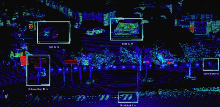
A Sense of Responsibility: Lidar Sensor Makers Build on NVIDIA DRIVE
When it comes to autonomous vehicle sensor innovation, it’s best to keep an open mind — and an open development platform.
That’s why NVIDIA DRIVE is the chosen platform on which the majority of these sensors run.
In addition to camera sensors, NVIDIA has long recognized that lidar is a crucial component to an autonomous vehicle’s perception stack. By emitting invisible lasers at incredibly fast speeds, lidar sensors can paint a detailed 3D picture from the signals that bounce back instantaneously.
These signals create “point clouds” that represent a three-dimensional view of the environment, allowing lidar sensors to provide the visibility, redundancy and diversity that contribute to safe automated and autonomous driving.
Most recently, lidar makers Baraja, Hesai, Innoviz, Magna and Ouster have developed their offerings to run on the NVIDIA DRIVE platform to deliver robust performance and flexibility to customers.
These sensors offer differentiated capabilities for AV sensing, from Innoviz’s lightweight, affordable and long-range solid-state lidar to Baraja’s long wavelength, long-range sensors.
“The open and flexible NVIDIA DRIVE platform is a game changer in allowing seamless integration of Innoviz lidar sensors in endless new and exciting opportunities,” said Innoviz CEO Omer Keilaf.
Ouster’s OS series of sensors offers high resolution as well as programmable fields of view to address autonomous driving use cases. It also provides a camera-like image with its digital lidar system-on-a-chip for greater perception capabilities.
Hesai’s latest Pandar128 sensor offers a 360-degree horizontal field of view with a detection range from 0.3 to 200 meters. In the vertical field of view, it uses denser beams to allow for high resolution in a focused region of interest. The low minimum range reduces the blind spot area close to and in front of the lidar sensor.
“The Hesai Pandar128’s resolution and detection range enable object detection at greater distances, making it an ideal solution for highly automated and autonomous driving systems,” said David Li, co-founder and CEO of Hesai. “Integrating our sensor with NVIDIA’s industry-leading DRIVE platform will provide an efficient pathway for AV developers.”
With the addition of these companies, the NVIDIA DRIVE ecosystem addresses every autonomous vehicle development need with verified hardware.
Plug and Drive
Typically, AV developers experiment with different variations of a sensor suite, modifying the number, type and placement of sensors. These configurations are necessary to continuously improve a vehicle’s capabilities and test new features.
An open, flexible compute platform can facilitate these iterations for effective autonomous vehicle development. And the industry agrees, with more than 60 sensor makers — from camera suppliers such as Sony, to radar makers like Continental, to thermal sensing companies such as FLIR — choosing to develop their products with the NVIDIA DRIVE AGX platform.
Along with the compute platform, NVIDIA provides the infrastructure to experience chosen sensor configurations with NVIDIA DRIVE Sim — an open simulation platform with plug-ins for third-party sensor models. As an end-to-end autonomous vehicle solutions provider, NVIDIA has long been a close partner to the leading sensor manufacturers.
“Ouster’s flexible digital lidar platform, including the new OS0-128 and OS2-128 lidar sensors, gives customers a wide variety of choices in range, resolution and field of view to fit in nearly any application that needs high-performance, low-cost 3D imaging,” said Angus Pacala, CEO of Ouster. “With Ouster as a member of the NVIDIA DRIVE ecosystem, our customers can plug and play our sensors easier than ever.”
Laser Focused
The NVIDIA DRIVE ecosystem includes a diverse set of lidar manufacturers — including Velodyne and Luminar as well as tier-1 suppliers — specializing in different features such as wavelength, signaling technique, field of view, range and resolution. This variety gives users flexibility as well as room for customization for their specific autonomous driving application.
The NVIDIA DriveWorks software development kit includes a sensor abstraction layer that provides a simple and unified interface that streamlines the bring-up process for new sensors on the platform. The interface saves valuable time and effort for developers as they test and validate different sensor configurations.

“To achieve maximum autonomous vehicle safety, a combination of sensor technologies including radar and lidar is required to see in all conditions. NVIDIA’s open ecosystem approach allows OEMs and tier 1s to select the safest and most cost-effective sensor configurations for each application,” said Jim McGregor, principal analyst at Tirias Research.
The NVIDIA DRIVE ecosystem gives autonomous vehicle developers the flexibility to select the right types of sensors for their vehicles, as well as iterate on configurations for different levels of autonomy. As an open AV platform with premier choices, NVIDIA DRIVE puts the automaker in the driver’s seat.
The post A Sense of Responsibility: Lidar Sensor Makers Build on NVIDIA DRIVE appeared first on The Official NVIDIA Blog.
How to deliver natural conversational experiences using Amazon Lex Streaming APIs
Natural conversations often include pauses and interruptions. During customer service calls, a caller may ask to pause the conversation or hold the line while they look up the necessary information before continuing to answer a question. For example, callers often need time to retrieve credit card details when making bill payments. Interruptions are also common. Callers may interrupt a human agent with an answer before the agent finishes asking the entire question (for example, “What’s the CVV code for your credit card? It is the three-digit code top right corner.…”). Just like conversing with human agents, a caller interacting with a bot may interrupt or instruct the bot to hold the line. Previously, you had to orchestrate such dialog on Amazon Lex by managing client attributes and writing code via an AWS Lambda function. Implementing a hold pattern required code to keep track of the previous intent so that the bot could continue the conversation. The orchestration of these conversations was complex to build and maintain, and impacted the time to market for conversational interfaces. Moreover, the user experience was disjointed because the properties of prompts such as ability to interrupt were defined in the session attributes on the client.
Amazon Lex’s new streaming conversation APIs allow you to deliver sophisticated natural conversations across different communication channels. You can now easily configure pauses, interruptions and dialog constructs while building a bot with the Wait and Continue and Interrupt features. This simplifies the overall design and implementation of the conversation and makes it easier to manage. By using these features, the bot builder can quickly enhance the conversational capability of virtual agents or IVR systems.
In the new Wait and Continue feature, the ability to put the conversation into a waiting state is surfaced during slot elicitation. You can configure the slot to respond with a “Wait” message such as “Sure, let me know when you’re ready” when a caller asks for more time to retrieve information. You can also configure the bot to continue the conversation with a “Continue” response based on defined cues such as “I’m ready for the policy ID. Go ahead.” Optionally, you can set a “Still waiting” prompt to play messages like “I’m still here” or “Let me know if you need more time.” You can set the frequency of these messages to play and configure a maximum wait time for user input. If the caller doesn’t provide any input within the maximum wait duration, Amazon Lex resumes the dialog by prompting for the slot. The following screenshot shows the wait and continue configuration options on the Amazon Lex console.

The Interrupt feature enables callers to barge-in while a prompt is played by the bot. A caller may interrupt the bot and answer a question before the prompt is completed. This capability is surfaced at the prompt level and provided as a default setting. On the Amazon Lex console, navigate to the Advanced Settings and under Slot prompts, enable the setting to allow users to interrupt the prompt.

After configuring these features, you can initiate a streaming interaction with the Lex bot by using the StartConversation API. The streaming capability enables you to capture user input, manage state transitions, handle events, and deliver a response required as part of a conversation. The input can be one of three types: audio, text, or DTMF, whereas the response can be either audio or text. The dialog progresses by eliciting an intent, populating any slots, confirming the intent, and finally closing the intent. Streaming allows intents to be defined based on different conversation states such as: InProgress, Waiting, Confirmed, Denied, Fulfilled, ReadyForFulfillment or Failed. A detailed list of different dialog and intents states, see the documentation for Amazon Lex intents.
The StartConversation API uses HTTP/2 for bidirectional communication between the client and Amazon Lex. Clients are expected to maintain a single long-running stream throughout the conversation and exchange required information with the server (and vice versa) via different events. To learn more about streaming for Amazon Lex bots, please refer the Lex streaming documentation.
Amazon Lex Streaming APIs in action
Let’s put all of this together in a bot. I first use the Amazon Lex console to configure a bot and then use the following sample telephony application to interact with the bot. For the purposes of this post, we use a simple bot to complete a bill payment with a credit card. Because callers often need time to retrieve their credit card details, we enable the wait and continue construct when eliciting the credit card number. We also set up a service-side interrupt to manage interruption.
The following is a sample conversation with our bot:
Caller: I’d like to make a payment on my account
Bot: Sure. Can we start off with your account ID?
Caller: Yes the account ID is 1234
Bot: Great. The balance due is $100. How much would you like to pay today?
Caller: $100
Bot: Ok. Can you share the 16-digit number on your credit card?
Caller: Can you wait a minute?
Bot: Sure—————- a few seconds later —————-
Bot: Let me know when ready. No rush.
—————- a few seconds later —————-
Caller: Ok I am back
Bot: Ok please go ahead
Caller: The credit card number is 1234 5678 1234 5678
Bot: Got it. Let me repeat that for you 1234 5678 1234 5678. Is that correct?
Caller: Yes
Bot: Ok. What’s the CVV code? You can find it in the top right on the signature panel on the back of the card.
Caller: 123
Bot: Awesome. I will go ahead and process the $100 payment on your account using the card ending in 5678.
Caller: Ok
Bot: The payment went through. Your confirmation code is 1234.
The first step is to build an Amazon Lex bot with intents to process payment and get balance on the account. The ProcessPayment intent elicits the information required to process the payment, such as the payment amount, credit card number, CVV code, and expiration date. The GetBalanceAmount intent provides the balance on the account. The FallbackIntent is triggered when the user input can’t be processed by either of the two configured intents.
Deploying the sample bot
To create the sample bot, complete the following steps. This creates an Amazon Lex bot called PaymentsBot.
- On the Amazon Lex console, choose Create Bot.
- In the Bot configuration section, give the bot the name
PaymentsBot. - Specify AWS Identity and Access Management (IAM) permissions and COPPA flag.
- Choose Next.
- Under Languages, choose English(US).
- Choose Done.
- Add the
ProcessPaymentandGetBalanceAmountintents to your bot. - For the
ProcessPaymentintent, add the following slots:PaymentAmountslot using the built-inAMAZON.Numberslot typeCreditCardNumberslot using the built-inAMAZON.AlphaNumericslot type- CVV slot using the built-in
AMAZON.Numberslot type ExpirationDateusing the built-inAMAZON.Datebuilt-in slot type
- Configure slot elicitation prompts for each slot.
- Configure a closing response for the
ProcessPaymentintent. - Similarly, add and configure slots and prompts for
GetBalanceAmountintents. - Choose Build to test your bot.
For more information about creating a bot, see the Lex V2 documentation.
Configuring Wait and Continue
- Choose the
ProcessPaymentintent and navigate to theCreditCardNumberslot. - Choose Advanced Settings to open the slot editor.
- Enable Wait and Continue for the slot.
- Provide the Wait, Still Waiting, and Continue responses.
- Save the intent and choose Build.
The bot is now configured to support the Wait and Continue dialog construct. Now let’s configure the client code. You can use a telephony application to interact with your Lex bot. You can download the code for setting up a telephony IVR interface via Twilio at the GitHub project. The link contains information to set up a telephony interface as well as a client application code to communicate between the telephony interface and Amazon Lex.
Now, let us review the client-side setup to use the bot configuration that we just enabled on the Amazon Lex console. The client application uses the Java SDK to capture payment information. In the beginning, you use the ConfigurationEvent to set up the conversation parameters. Then, you start sending an input event (AudioInputEvent, TextInputEvent or DTMFInputEvent) to send user input to the bot depending on the input type. When sending audio data, you would need to send multiple AudioInputEvent events, with each event containing a slice of the data.
The service first responds with TranscriptEvent to give transcription, then sends the IntentResultEvent to surface the intent classification results. Subsequently, Amazon Lex sends a response event (TextResponseEvent or AudioResponseEvent) that contains the response to play back to caller. If the caller requests the bot to hold the line, the intent is moved to the Waiting state and Amazon Lex sends another set of TranscriptEvent, IntentResultEvent and a response event. When the caller requests to continue the conversation, the intent is set to the InProgress state and the service sends another set of TranscriptEvent, IntentResultEvent and a response event. While the dialog is in the Waiting state, Amazon Lex responds with a set of IntentResultEvent and response event for every “Still waiting” message (there is no transcript event for server-initiated responses). If the caller interrupts the bot prompt at any time, Amazon Lex returns a PlaybackInterruptionEvent.
Let’s walk through the main elements of the client code:
- Create the Amazon Lex client:
AwsCredentialsProvider awsCredentialsProvider = StaticCredentialsProvider .create(AwsBasicCredentials.create(accessKey, secretKey)); LexRuntimeV2AsyncClient lexRuntimeServiceClient = LexRuntimeV2AsyncClient.builder() .region(region) .credentialsProvider(awsCredentialsProvider) .build(); - Create a handler to publish data to server:
EventsPublisher eventsPublisher = new EventsPublisher();
- Create a handler to process bot responses:
public class BotResponseHandler implements StartConversationResponseHandler {

    private static final Logger LOG = Logger.getLogger(BotResponseHandler.class);


    @Override
    public void responseReceived(StartConversationResponse startConversationResponse) {
        LOG.info("successfully established the connection with server. request id:" + startConversationResponse.responseMetadata().requestId()); // would have 2XX, request id.
    }

    @Override
    public void onEventStream(SdkPublisher<StartConversationResponseEventStream> sdkPublisher) {

        sdkPublisher.subscribe(event -> {
            if (event instanceof PlaybackInterruptionEvent) {
                handle((PlaybackInterruptionEvent) event);
            } else if (event instanceof TranscriptEvent) {
                handle((TranscriptEvent) event);
            } else if (event instanceof IntentResultEvent) {
                handle((IntentResultEvent) event);
            } else if (event instanceof TextResponseEvent) {
                handle((TextResponseEvent) event);
            } else if (event instanceof AudioResponseEvent) {
                handle((AudioResponseEvent) event);
            }
        });
    }

    @Override
    public void exceptionOccurred(Throwable throwable) {
        LOG.error(throwable);
        System.err.println("got an exception:" + throwable);
    }

    @Override
    public void complete() {
        LOG.info("on complete");
    }

    private void handle(PlaybackInterruptionEvent event) {
        LOG.info("Got a PlaybackInterruptionEvent: " + event);

        LOG.info("Done with a  PlaybackInterruptionEvent: " + event);
    }

    private void handle(TranscriptEvent event) {
        LOG.info("Got a TranscriptEvent: " + event);
    }


    private void handle(IntentResultEvent event) {
        LOG.info("Got an IntentResultEvent: " + event);

    }

    private void handle(TextResponseEvent event) {
        LOG.info("Got an TextResponseEvent: " + event);

    }

    private void handle(AudioResponseEvent event) {//synthesize speech
        LOG.info("Got a AudioResponseEvent: " + event);
    }

}
- Initiate the connection with the bot:
StartConversationRequest.Builder startConversationRequestBuilder = StartConversationRequest.builder() .botId(botId) .botAliasId(botAliasId) .localeId(localeId); // configure the conversation mode with bot (defaults to audio) startConversationRequestBuilder = startConversationRequestBuilder.conversationMode(ConversationMode.AUDIO); // assign a unique identifier for the conversation startConversationRequestBuilder = startConversationRequestBuilder.sessionId(sessionId); // build the initial request StartConversationRequest startConversationRequest = startConversationRequestBuilder.build(); CompletableFuture<Void> conversation = lexRuntimeServiceClient.startConversation( startConversationRequest, eventsPublisher, botResponseHandler); - Establish the configurable parameters via
ConfigurationEvent:public void configureConversation() { String eventId = "ConfigurationEvent-" + eventIdGenerator.incrementAndGet(); ConfigurationEvent configurationEvent = StartConversationRequestEventStream .configurationEventBuilder() .eventId(eventId) .clientTimestampMillis(System.currentTimeMillis()) .responseContentType(RESPONSE_TYPE) .build(); eventWriter.writeConfigurationEvent(configurationEvent); LOG.info("sending a ConfigurationEvent to server:" + configurationEvent); } - Send audio data to server:
public void writeAudioEvent(ByteBuffer byteBuffer) { String eventId = "AudioInputEvent-" + eventIdGenerator.incrementAndGet(); AudioInputEvent audioInputEvent = StartConversationRequestEventStream .audioInputEventBuilder() .eventId(eventId) .clientTimestampMillis(System.currentTimeMillis()) .audioChunk(SdkBytes.fromByteBuffer(byteBuffer)) .contentType(AUDIO_CONTENT_TYPE) .build(); eventWriter.writeAudioInputEvent(audioInputEvent); } - Manage interruptions on the client side:
private void handle(PlaybackInterruptionEvent event) { LOG.info("Got a PlaybackInterruptionEvent: " + event); callOperator.pausePlayback(); LOG.info("Done with a PlaybackInterruptionEvent: " + event); } - Enter the code to disconnect the connection:
public void disconnect() {

    String eventId = "DisconnectionEvent-" + eventIdGenerator.incrementAndGet();

    DisconnectionEvent disconnectionEvent = StartConversationRequestEventStream
            .disconnectionEventBuilder()
            .eventId(eventId)
            .clientTimestampMillis(System.currentTimeMillis())
            .build();

    eventWriter.writeDisconnectEvent(disconnectionEvent);

    LOG.info("sending a DisconnectionEvent to server:" + disconnectionEvent);
}
You can now deploy the bot on your desktop to test it out.
Things to know
The following are a couple of important things to keep in mind when you’re using the Amazon Lex V2 Console and APIs:
- Regions and languages – The Streaming APIs are available in all existing Regions and support all current languages.
- Interoperability with Lex V1 console – Streaming APIs are only available in the Lex V2 console and APIs.
- Integration with Amazon Connect – As of this writing, Lex V2 APIs are not supported on Amazon Connect. We plan to provide this integration as part of our near-term roadmap.
- Pricing – Please see the details on the Lex pricing page.
Try it out
Amazon Lex Streaming API is available now and you can start using it today. Give it a try, design a bot, launch it and let us know what you think! To learn more, please see the Lex streaming API documentation.
About the Authors
 Esther Lee is a Product Manager for AWS Language AI Services. She is passionate about the intersection of technology and education. Out of the office, Esther enjoys long walks along the beach, dinners with friends and friendly rounds of Mahjong.
 Swapandeep Singh is an engineer with Amazon Lex team. He works on making interactions with bot smoother and more human-like. Outside of work, he likes to travel and learn about different cultures.
Stabilizing Live Speech Translation in Google Translate
Posted by Naveen Arivazhagan, Senior Software Engineer and Colin Cherry, Staff Research Scientist, Google Research
The transcription feature in the Google Translate app may be used to create a live, translated transcription for events like meetings and speeches, or simply for a story at the dinner table in a language you don’t understand. In such settings, it is useful for the translated text to be displayed promptly to help keep the reader engaged and in the moment.
However, with early versions of this feature the translated text suffered from multiple real-time revisions, which can be distracting. This was because of the non-monotonic relationship between the source and the translated text, in which words at the end of the source sentence can influence words at the beginning of the translation.
 |
| Transcribe (old) — Left: Source transcript as it arrives from speech recognition. Right: Translation that is displayed to the user. The frequent corrections made to the translation interfere with the reading experience. |
Today, we are excited to describe some of the technology behind a recently released update to the transcribe feature in the Google Translate app that significantly reduces translation revisions and improves the user experience. The research enabling this is presented in two papers. The first formulates an evaluation framework tailored to live translation and develops methods to reduce instability. The second demonstrates that these methods do very well compared to alternatives, while still retaining the simplicity of the original approach. The resulting model is much more stable and provides a noticeably improved reading experience within Google Translate.
 |
| Transcribe (new) — Left: Source transcript as it arrives from speech recognition. Right: Translation that is displayed to the user. At the cost of a small delay, the translation now rarely needs to be corrected. |
Evaluating Live Translation
Before attempting to make any improvements, it was important to first understand and quantifiably measure the different aspects of the user experience, with the goal of maximizing quality while minimizing latency and instability. In “Re-translation Strategies For Long Form, Simultaneous, Spoken Language Translation”, we developed an evaluation framework for live-translation that has since guided our research and engineering efforts. This work presents a performance measure using the following metrics:
- Erasure: Measures the additional reading burden on the user due to instability. It is the number of words that are erased and replaced for every word in the final translation.
- Lag: Measures the average time that has passed between when a user utters a word and when the word’s translation displayed on the screen becomes stable. Requiring stability avoids rewarding systems that can only manage to be fast due to frequent corrections.
- BLEU score: Measures the quality of the final translation. Quality differences in intermediate translations are captured by a combination of all metrics.
It is important to recognize the inherent trade-offs between these different aspects of quality. Transcribe enables live-translation by stacking machine translation on top of real-time automatic speech recognition. For each update to the recognized transcript, a fresh translation is generated in real time; several updates can occur each second. This approach placed Transcribe at one extreme of the 3 dimensional quality framework: it exhibited minimal lag and the best quality, but also had high erasure. Understanding this allowed us to work towards finding a better balance.
Stabilizing Re-translation
One straightforward solution to reduce erasure is to decrease the frequency with which translations are updated. Along this line, “streaming translation” models (for example, STACL and MILk) intelligently learn to recognize when sufficient source information has been received to extend the translation safely, so the translation never needs to be changed. In doing so, streaming translation models are able to achieve zero erasure.
The downside with such streaming translation models is that they once again take an extreme position: zero erasure necessitates sacrificing BLEU and lag. Rather than eliminating erasure altogether, a small budget for occasional instability may allow better BLEU and lag. More importantly, streaming translation would require retraining and maintenance of specialized models specifically for live-translation. This precludes the use of streaming translation in some cases, because keeping a lean pipeline is an important consideration for a product like Google Translate that supports 100+ languages.
In our second paper, “Re-translation versus Streaming for Simultaneous Translation”, we show that our original “re-translation” approach to live-translation can be fine-tuned to reduce erasure and achieve a more favorable erasure/lag/BLEU trade-off. Without training any specialized models, we applied a pair of inference-time heuristics to the original machine translation models — masking and biasing.
The end of an on-going translation tends to flicker because it is more likely to have dependencies on source words that have yet to arrive. We reduce this by truncating some number of words from the translation until the end of the source sentence has been observed. This masking process thus trades latency for stability, without affecting quality. This is very similar to delay-based strategies used in streaming methods such as Wait-k, but applied only during inference and not during training.
Neural machine translation often “see-saws” between equally good translations, causing unnecessary erasure. We improve stability by biasing the output towards what we have already shown the user. On top of reducing erasure, biasing also tends to reduce lag by stabilizing translations earlier. Biasing interacts nicely with masking, as masking words that are likely to be unstable also prevents the model from biasing toward them. However, this process does need to be tuned carefully, as a high bias, along with insufficient masking, may have a negative impact on quality.
The combination of masking and biasing, produces a re-translation system with high quality and low latency, while virtually eliminating erasure. The table below shows how the metrics react to the heuristics we introduced and how they compare to the other systems discussed above. The graph demonstrates that even with a very small erasure budget, re-translation surpasses zero-flicker streaming translation systems (MILk and Wait-k) trained specifically for live-translation.
| System | BLEU | Lag (seconds) |
Erasure | |||
| Re-translation (Transcribe old) |
20.4 | 4.1 | 2.1 | |||
| + Stabilization (Transcribe new) |
20.2 | 4.1 | 0.1 |
| Evaluation of re-translation on IWSLT test 2018 Engish-German (TED talks) with and without the inference-time stabilization heuristics of masking and biasing. Stabilization drastically reduces erasure. Translation quality, measured in BLEU, is very slightly impacted due to biasing. Despite masking, the effective lag remains the same because the translation stabilizes sooner. |
 |
| Comparison of re-translation with stabilization and specialized streaming models (Wait-k and MILk) on WMT 14 English-German. The BLEU-lag trade-off curve for re-translation is obtained via different combinations of bias and masking while maintaining an erasure budget of less than 2 words erased for every 10 generated. Re-translation offers better BLEU / lag trade-offs than streaming models which cannot make corrections and require specialized training for each trade-off point. |
Conclusion
The solution outlined above returns a decent translation very quickly, while allowing it to be revised as more of the source sentence is spoken. The simple structure of re-translation enables the application of our best speech and translation models with minimal effort. However, reducing erasure is just one part of the story — we are also looking forward to improving the overall speech translation experience through new technology that can reduce lag when the translation is spoken, or that can enable better transcriptions when multiple people are speaking.
Certifiably Fast: Top OEMs Debut World’s First NVIDIA-Certified Systems Built to Crush AI Workloads
AI, the most powerful technology of our time, demands a new generation of computers tuned and tested to drive it forward.
Starting today, data centers can get boot up a new class of accelerated servers from our partners to power their journey into AI and data analytics. Top system makers are delivering the first wave of NVIDIA-Certified Systems, the industry’s only servers tested for modern workloads.
These systems speed AI thanks to NVIDIA’s latest GPUs riding NVIDIA Mellanox networks. They spin up machine learning techniques that unearth insights from growing mounds of corporate data, gems that traditional systems miss.
Dell Technologies, GIGABYTE, Hewlett Packard Enterprise, Inspur and Supermicro are all shipping certified servers today. NVIDIA is collaborating with top OEMs around the world to drive AI forward across every industry.
The first systems off the line using NVIDIA A100 Tensor Core GPUs include:
- Dell EMC PowerEdge R7525 and R740 rack servers
- GIGABYTE R281-G30, R282-Z96, G242-Z11, G482-Z54, G492-Z51 systems
- HPE Apollo 6500 Gen10 System and HPE ProLiant DL380 Gen10 Server
- Inspur NF5488A5
- Supermicro A+ Server AS -4124GS-TNR and AS -2124GQ-NART
They all carry the NVIDIA-Certified Systems badge that gives customers confidence they’re buying systems that meet NVIDIA’s best design practices. That means they can tackle the toughest tasks in machine learning, data analytics and more.

A Tipping Point for Enterprise AI
The systems arrive as leading corporations are getting traction in AI.
American Express is using the latest AI models for real-time fraud detection. Ford taps generative adversarial networks to generate data it needs to test self-driving cars. And Dominos applies AI to improve predictions of when orders will be ready for the 3 billion pizzas it delivers every year.
They are among many companies plugging into a powerful new form of computing, born on the web and now spreading into sectors from retail and logistics to banking and healthcare.
Gartner estimates 37 percent of all organizations have AI in production today and predicts that will double to 75 percent by 2024.
Scaling a Big Data Mountain
Companies seek strategic insights hidden in a rising mountain of data. Walmart, for example, processes more than 2.5 petabytes of data every hour.
AI models to sift through that data have grown in size by nearly 30,000x in just five years, driving the need for accelerated computing. And the diversity of models and workloads using them continues to expand, so businesses need the flexibility of GPUs.
The rising tide of data and the expanding AI models to sift through it are spawning an exponential increase in network traffic both in the data center and at the network’s edge. To cope, companies need a secure, reliable and high-speed infrastructure that scales efficiently.
Acing the Test for AI
NVIDIA-Certified Systems deliver the performance, programmability and secure throughput enterprise AI needs. They combine the computing power of GPUs based on the NVIDIA Ampere architecture with secure, high-speed NVIDIA Mellanox networking.
To pass the certification, the systems are tested across a broad range of workloads, from jobs that require multiple compute nodes to tasks that only need part of the power of a single GPU.
The systems are optimized to run AI applications from the NGC catalog, NVIDIA’s hub for GPU-optimized applications.
NGC is also the home for an expanding set of software development kits that bring AI to vertical markets such as healthcare (Clara) and robotics (Isaac). In addition, it holds frameworks that help companies get started in emerging use cases like recommendation systems (Merlin) and intelligent video analytics (Metropolis).
Specifically, NVIDIA-Certified Systems must pass tests on:
- Deep learning training and inference
- Machine learning algorithms
- Intelligent video analytics
- Network and storage offload
The tests focus on real-world use cases. They use popular AI frameworks and containers, all available in the NGC catalog.
As a result, NVIDIA-Certified Systems let every company access the same hardware and software behind some of the most powerful AI computers on the planet.
All of the world’s largest cloud service providers and eight of the world’s top 10 supercomputers are powered by NVIDIA technology. And NVIDIA-based systems lead in AI benchmarks such as MLPerf.
A Peek Under the Hood
NVIDIA-Certified Systems include powerful data center servers with as many as eight A100 GPUs and high-speed InfiniBand or Ethernet network adapters. Others are mainstream AI systems tailored to run AI at the edge of the corporate network.
OEMs certify the systems using NVIDIA Mellanox cables, switches and network cards such as ConnectX-6 InfiniBand or Ethernet adapters and BlueField-2 DPUs. In addition to high throughput at low latency, these adapters support multiple layers of security from a hardware root of trust at boot time to connection tracking for applications.
Every system was certified using either an NVIDIA Mellanox 8700 HDR 200G InfiniBand switch or the Mellanox SN3700 Ethernet switch.
All NVIDIA-Certified Systems are available with enterprise support across the full software stack, including support for open source code. That’s because we want to ensure enterprises across all vertical markets can quickly enjoy the benefits of AI.
With the latest systems from Dell Technologies, GIGABYTE, HPE, Inspur, and Supermicro, every company can start its own journey to enterprise AI.
To date, 14 servers from six systems makers are certified and ready to provide accelerated computing. They are among 70 systems from at least 11 system makers engaged in the program.
Stay tuned for news of more NVIDIA-Certified Systems from more partners.
![]()
The post Certifiably Fast: Top OEMs Debut World’s First NVIDIA-Certified Systems Built to Crush AI Workloads appeared first on The Official NVIDIA Blog.