Introduction
Machine learning models are susceptible to learning irrelevant patterns.
In other words, they rely on some spurious features that we humans know
to avoid. For example, assume that you are training a model to predict
whether a comment is toxic on social media platforms. You would expect
your model to predict the same score for similar sentences with
different identity terms. For example, “some people are Muslim” and
“some people are Christian” should have the same toxicity score.
However, as shown in 1, training a convolutional
neural net leads to a model which assigns different toxicity scores to
the same sentences with different identity terms. Reliance on spurious
features is prevalent among many other machine learning models. For
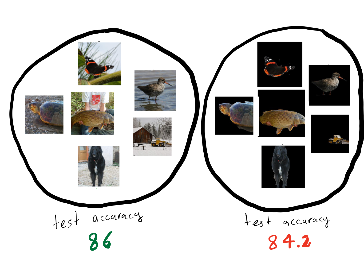
instance, 2 shows that state of the art models in object
recognition like Resnet-50 3 rely heavily on background, so
changing the background can also change their predictions .
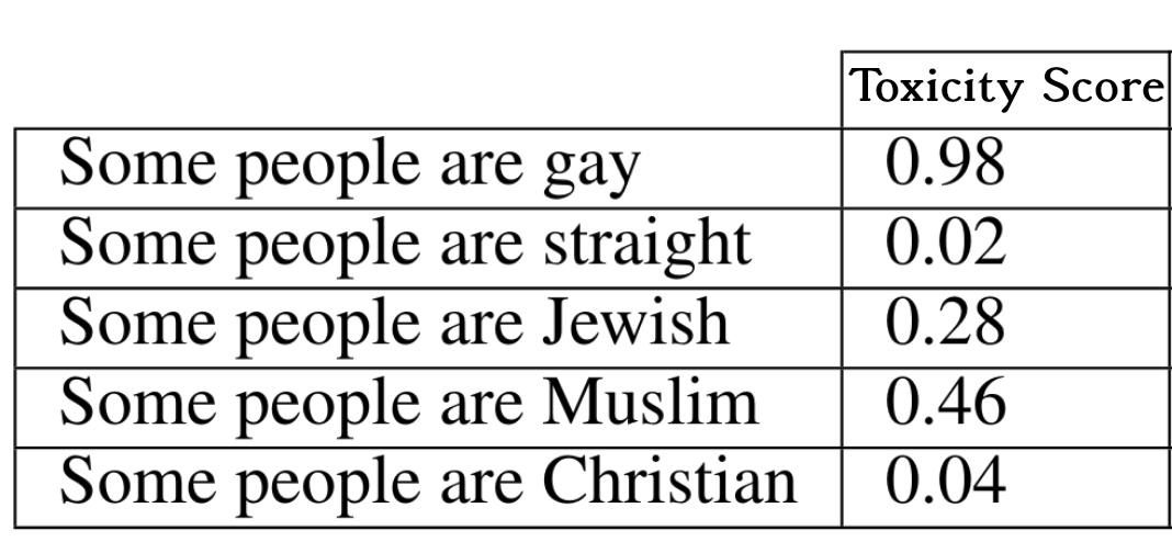

(Left) Machine learning models assign different toxicity scores to the
same sentences with different identity terms.
(Right) Machine learning models make different predictions on the same
object against different backgrounds.
Machine learning models rely on spurious features such as background in an image or identity terms in a comment. Reliance on spurious features conflicts with fairness and robustness goals.
Of course, we do not want our model to rely on such spurious features
due to fairness as well as robustness concerns. For example, a model’s
prediction should remain the same for different identity terms
(fairness); similarly its prediction should remain the same with
different backgrounds (robustness). The first instinct to remedy this
situation would be to try to remove such spurious features, for example,
by masking the identity terms in the comments or by removing the
backgrounds from the images. However, removing spurious features can
lead to drops in accuracy at test time 45. In this
blog post, we explore the causes of such drops in accuracy.
There are two natural explanations for accuracy drops:
- Core (non-spurious) features can be noisy or not expressive enough
so that even an optimal model has to use spurious features to
achieve the best accuracy
678. - Removing spurious features can corrupt the core features
910.
One valid question to ask is whether removing spurious features leads to
a drop in accuracy even in the absence of these two reasons. We answer
this question affirmatively in our recently published work in ACM Conference on Fairness, Accountability, and Transparency (ACM FAccT) 11. Here, we explain our results.
Removing spurious features can lead to drop in accuracy even when spurious features are removed properly and core features exactly determine the target!


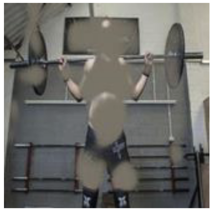
(Left) When core features are not representative (blurred image), the
spurious feature (the background) provides extra information to identify
the object. (Right) Removing spurious features (gender
information) in the sport prediction task has corrupted other core
features (the weights and the bar).
Before delving into our result, we note that understanding the reasons
behind the accuracy drop is crucial for mitigating such drops. Focusing
on the wrong mitigation method fails to address the accuracy drop.
Before trying to mitigate the accuracy drop resulting from the removal of the spurious features, we must understand the reasons for the drop.
| Previous work | Previous work | This work | |
|---|---|---|---|
 |
 |
 |
|
| Removing spurious features causes drops in accuracy because… | core features are noisy and not sufficiently expressive. | spurious features are not removed properly and thus corrupt core features. | a lack of training data causes spurious connections between some features and the target. |
| We can mitigate such drops by… | focusing on collecting more expressive features (e.g., high-resolution images) | focusing on more accurate methods for removing spurious features. | focusing on collecting more diverse training data. We show how to leverage unlabeled data to achieve such diversity. |
This work in a nutshell:
- We study overparameterized models that fit training data perfectly.
- We compare the “core model” that only uses core features (non-spurious) with the “full model” that uses both core features and spurious features.
- Using the spurious feature, the full model can fit training data with a smaller norm.
- In the overparameterized regime, since the number of training examples is less than the number of features, there are some directions of data variation that are not observed in the training data (unseen directions).
- Though both models fit the training data perfectly, they have different “assumptions’’ for the unseen directions. This difference can lead to
- Drop in accuracy
- Affecting different test distributions (we also call them groups) disproportionately (increasing accuracy in some while decreasing accuracy in others).

Noiseless Linear Regression
Over the last few years, researchers have observed some surprising
phenomena about deep networks that conflict with classical machine
learning. For example, training models to zero training loss leads to
better generalization instead of overfitting 12. A line
of work 1314 found that these unintuitive
results happen even for simple models such as linear regression if the
number of features are greater than the number of training data, known
as the overparameterized regime.
Accuracy drops due to the removal of spurious features is also
unintuitive. Classical machine learning tells us that removing spurious
features should decrease generalization error (since these features are,
by definition, irrelevant for the task). Analogous to the mentioned
work, we will explain this unintuitive result in overparameterized
linear regression as well.
Accuracy drop due to removal of the spurious feature can be explained in overparameterized linear regression.
Let’s first formalize the noiseless linear regression setup. Recall
that we are going to study a setup in which the target is completely
determined by the core features, and the spurious feature is a single
feature that can be removed perfectly without affecting predictive
performance. Formally, we assume there are (d) core features
(z in mathbb{R}^d) that determine the target (y in
mathbb{R}) perfectly, i.e., ( y = {theta^star}^top z).
In addition, we assume there is a single spurious feature (s) that
can also be determined by the core features (s =
{beta^star}^top z). Note that the spurious feature can have
information about features that determine the target or it can be
completely unrelated to the target (i.e., for all (i),
(beta^star_i theta^star_i=0)).
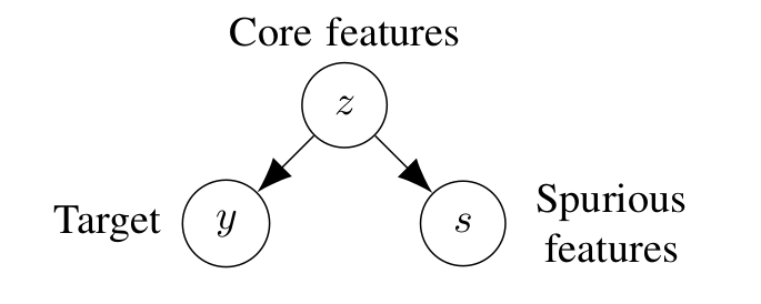
We consider a setup where target ((y)) is a deterministic function
of core features ((z)). In addition, there is a spurious feature
((s)) that can also be determined by the core feature. We compare
two models, the core model that only uses (z) to predict (y) and the full model which uses both (z) and (s) to predict
(y).
We consider two models:
- Core model that only uses the core features (z) to predict the
target (y), and it is parametrized by
({theta^text{-s}}). For a data point with core features
(z), its prediction is (hat y =
{theta^text{-s}}^top z). - Full model that uses the core features (z) and also uses the
spurious feature (s), and it is parametrized by
({theta^text{+s}}), and (w), For a data point with
core feature (z) and a spurious feature (s), its
prediction is (hat y = {theta^text{+s}}^top z + ws).
In this setup, the mentioned two reasons that naturally can cause
accuracy drop after removing the spurious feature (depicted in the table
above) do not exist.
- The spurious feature (s) adds no information about the target
(y) beyond what already exists in the core features
(z) (reason 1), - Removing (s) does not corrupt (z) (reason 2).
Motivated by recent work in deep learning, which speculates that
gradient descent converges to the minimum-norm solution that fits
training data perfectly 15, we consider the
minimum-norm solution.
- Training data: We assume we have (n < d) triples of
((z_i, s_i, y_i)) - Test data: We assume core features in the test data are from a
distribution with covariance matrix (Sigma =
mathbb{E}[zz^top]) (we use group and test data distribution
exchangeably).
In this simple setting, one might conjecture that removing the spurious
feature should only help accuracy. However, we show that this is not
always the case. We exactly characterize the test distributions that are
negatively affected by removing spurious features, as well as the ones
that are positively affected by it.
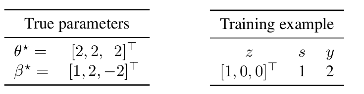
Example
Let’s first look at a simple example with only one training data and
three core features ((z_1, z_2) and (z_3)). Let the true
parameters (theta^star =[2,2,2]^top) which results in
(y=2), and let the spurious feature parameter ({beta^star}
= [1,2,-2]^top) which results in (s=1).
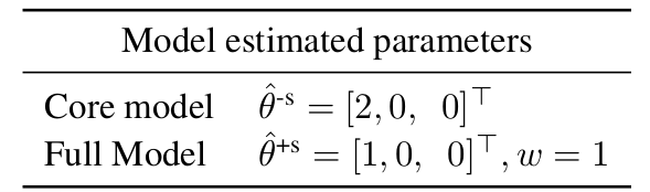
First, note that the smallest L2-norm vector that can fit the training
data for the core model is ({theta^text{-s}}=[2,0,0]). On
the other hand, in the presence of the spurious feature, the full model
can fit the training data perfectly with a smaller norm by assigning
weight (1) for the feature (s)
((|{theta^text{-s}}|_2^2 = 4) while
(|{theta^text{+s}}|_2^2 + w^2 = 2 < 4)).
Generally, in the overparameterized regime, since the number of training
examples is less than the number of features, there are some directions
of data variation that are not observed in the training data. In this
example, we do not observe any information about the second and third
features. The core model assigns weight (0) to the unseen
directions (weight (0) for the second and third features in this
example). However, the non-zero weight for the spurious feature leads to
a different assumption for the unseen directions. In particular, the
full model does not assign weight (0) to the unseen directions.
Indeed, by substituting (s) with ({beta^star}^top
z), we can view the full model as not using (s) but
implicitly assigning weight (beta^star_2=2) to the second
feature and (beta^star_3=-2) to the third feature (unseen
directions at training).
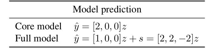
Let’s now look at different examples and the prediction of these two
models:
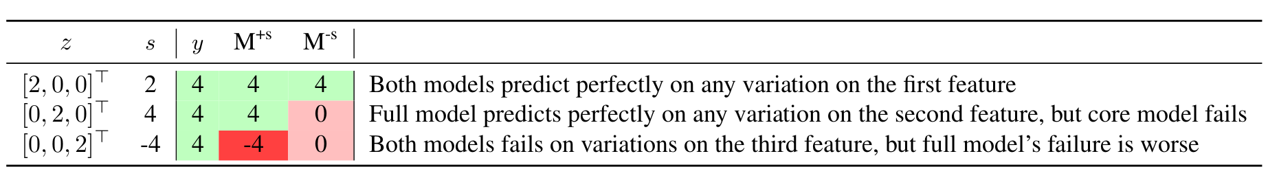
In this example, removing (s) reduces the error for a test
distribution with high deviations from zero on the second feature,
whereas removing (s) increases the error for a test distribution
with high deviations from zero on the third feature.
Main result
As we saw in the previous example, by using the spurious feature, the
full model incorporates ({beta^star}) into its estimate. The
true target parameter ((theta^star)) and the true spurious
feature parameters (({beta^star})) agree on some of the
unseen directions and do not agree on the others. Thus, depending on
which unseen directions are weighted heavily in the test time, removing
(s) can increase or decrease the error.
More formally, the weight assigned to the spurious feature is
proportional to the projection of (theta^star) on
({beta^star}) on the seen directions. If this number is close
to the projection of (theta^star) on ({beta^star})
on the unseen directions (in comparison to 0), removing (s)
increases the error, and it decreases the error otherwise. Note that
since we are assuming noiseless linear regression and choose models that
fit training data, the model predicts perfectly in the seen directions
and only variations in unseen directions contribute to the error.
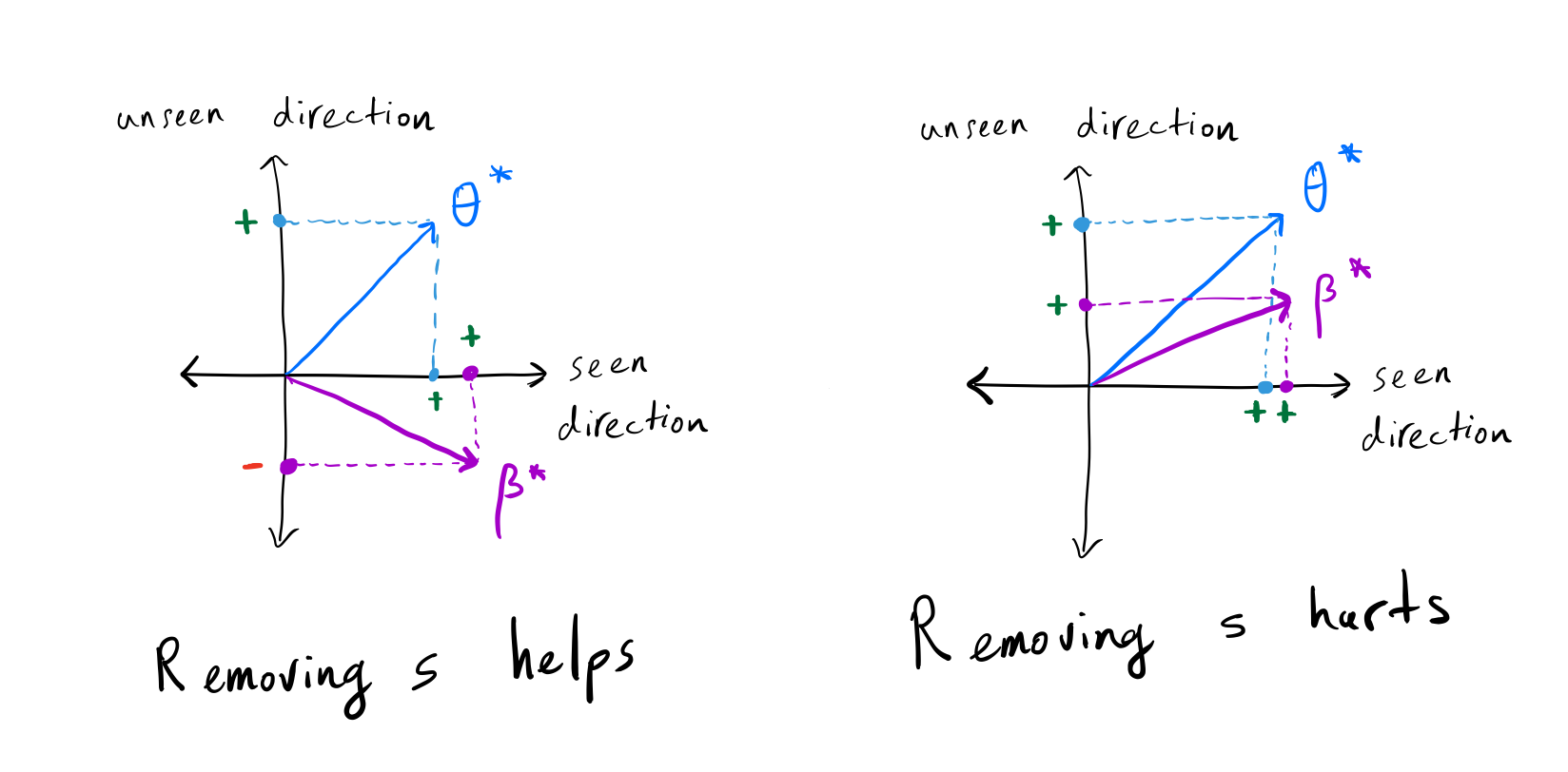
(Left) The projection of (theta^star) on
(beta^star) is positive in the seen direction, but it is
negative in the unseen direction; thus, removing (s) decreases the
error. (Right) The projection of (theta^star) on
(beta^star) is similar in both seen and unseen directions;
thus, removing (s) increases the error.
Drop in accuracy in test time depends on the relationship between the true target parameter ((theta^star)) and the true spurious feature parameters (({beta^star})) in the seen directions and unseen direction.
Let’s now formalize the conditions under which removing the spurious
feature ((s)) increases the error. Let (Pi =
Z(ZZ^top)^{-1}Z) denote the column space of training data (seen
directions), thus (I-Pi) denotes the null space of training data
(unseen direction). The below equation determines when removing the
spurious feature decreases the error.
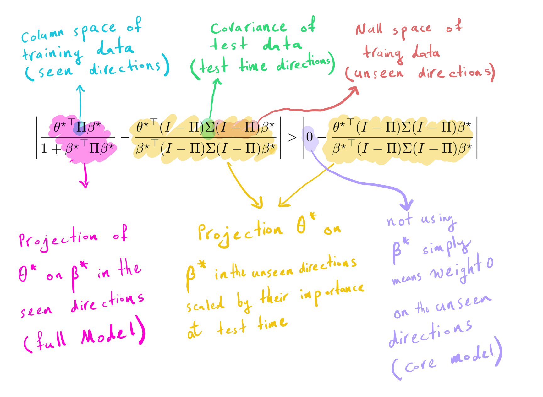
The left side is the difference between the projection of (theta^star) on (beta^star) in the seen direction
with their projection in the unseen direction scaled by test time
covariance. The right side is the difference between 0 (i.e., not using
spurious features) and the projection of (theta^star) on
(beta^star) in the unseen direction scaled by test time
covariance. Removing (s) helps if the left side is greater than
the right side.
Experiments
While the theory applies only to linear models, we now show that in
non-linear models trained on real-world datasets, removing a spurious
feature reduces the accuracy and affects groups disproportionately.
Datasets. We are going to study the CelebA dataset 16 which
contains photos of celebrities along with 40 different attributes.
footnote{See our paper for the results on the
comment-toxicity-detection and MNIST datasets} We choose wearing
lipstick (indicating if a celebrity is wearing lipstick) as the target
and wearing earrings (indicating if a celebrity is wearing earrings) as
the spurious feature.
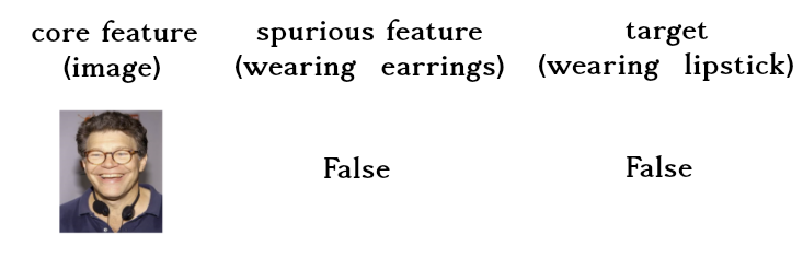
Note that although wearing earrings is correlated with wearing lipstick,
we expect our model to not change its prediction if we tell the model
the person is wearing earrings.
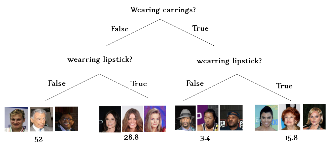
In the CelebA dataset wearing earrings is correlated with wearing
lipstick. In this dataset, if a celebrity wears earrings, it is almost
five times more likely that they will wear lipstick than not wearing
lipstick. Similarly, if a celebrity does not wear earrings, it is
almost two times more likely for them not to wear lipstick than wearing
lipstick.
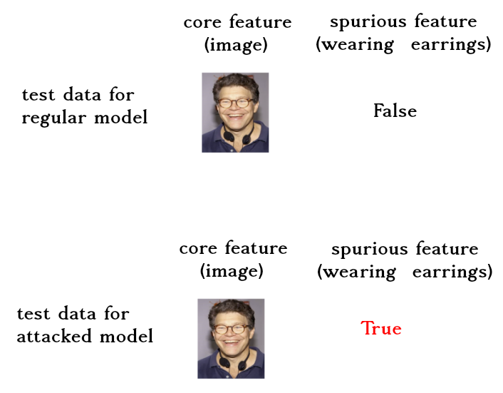
Setup. We train a two-layer neural network with 128 hidden units. We
flatten the picture and concatenate the binary variable of wearing
earrings to it (we tuned a multiplier for it). We also want to know how
much each model relies on the spurious feature. In other words, we want
to know how much the model prediction changes as we change the wearing
earrings variable. We call this attacking the model (i.e, swapping the
value of the binary feature of wearing earrings). We run each experiment
50 times and report the average.
Results. The below diagram shows the accuracy of different models, and
their accuracies when they are attacked. Note that, because our attack
focuses on the spurious feature, the core model’s accuracy will remain
the same.
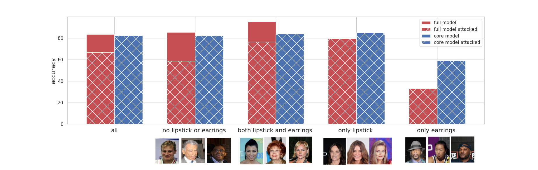
Removal of the wearing lipstick decreases the overall accuracy. The
decrease in accuracy is not monotonic among different groups. The
accuracy has decreased in the group where people are not wearing
lipstick or earrings and in the group that they both have lipstick and
earrings. On the other hand, accuracy increases for the group that only
wears one of them.
Let’s break down the diagram and analyze each section.
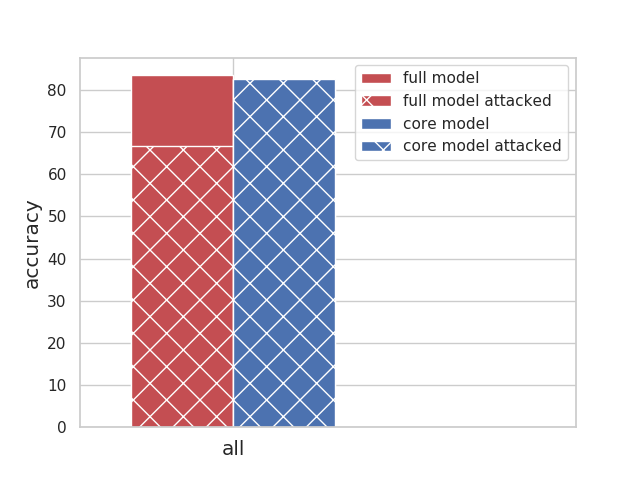 |
All celebrities together: have a reasonable accuracy of 82% The overall accuracy drops 1% when we remove the spurious feature (core model accuracy). The full model relies on the spurious feature a lot, thus attacking the full model leads to a ~ 17% drop in overall accuracy. |
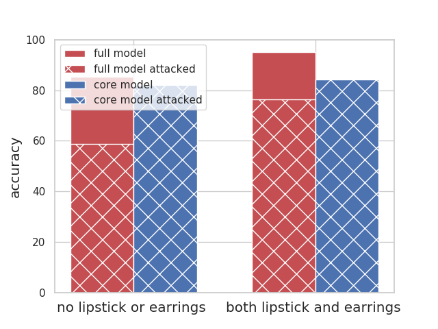 |
The celebrities who follow the stereotype (people who do not have earrings or lipstick, and people who wear both) have a good accuracy overall (both above 85%); The accuracy of both groups drop as we remove the wearing earrings (i.e., core model accuracy). Using the spurious feature helps their accuracy, thus attacking the full model leads to a ~30% drop in their accuracy. |
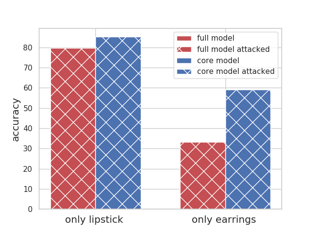 |
The celebrities who do not follow the stereotypes have a very low accuracy; this is especially worse for people who only wear earrings (33% accuracy in comparison to the average of 85%). Removing the wearing earring increases their accuracy substantially. Using the spurious feature does not help their accuracy, thus attacking the full model does not change accuracy for these groups. |
In non-linear models trained on real-world datasets, removing a spurious feature reduces the accuracy and affects groups disproportionately.
Q&A (Other results):
I know about my problem setting, and I am certain that disjoint features
determine the target and the spurious feature (i.e., for all (i),
(theta^star_ibeta^star_i=0)). Can I be sure that my
model will not rely on the spurious feature, and removing the spurious
feature definitely reduces the error? No! Actually, for any
(theta^star) and ({beta^star}), we can construct a
training set and two test sets with (theta^star) and
({beta^star}) as the true parameters and the spurious feature
parameter, such that removing the spurious feature reduces the error in
one but increases the error in the other one (see Corollary 1 in our
paper).
I am collecting a balanced dataset such that the spurious feature and
the target are completely independent (i.e., (p[y,s]= p[y]p[s])).
Can I be sure that my model will not rely on the spurious feature, and
removing the spurious feature definitely reduces the error?
No! for any
(S in mathbb{R}^n) and (Y in mathbb{R}^n), we can
generate a training set and two test sets with (S) and (Y)
as their spurious feature and targets, respectively, such that removing
the spurious feature reduces the error in one but increases the error in
the other (see Corollary 2 in our paper).
What happens when we have many spurious features? Good question! Let’s
say (s_1) and (s_2) are two spurious features. We show
that:
- Removing (s_1) makes the model more sensitive against
(s_2), and - If a group has high error because of the new assumption about unseen
direction enforced by using (s_2), then it will have an even
higher error by removing (s_1).
(See Proposition 3 in our paper).
Is it possible to have the same model (a model with the same assumptions
on unseen directions as the full model) without relying on the spurious
feature (i.e., be robust against the spurious feature)? Yes! You can
recover the same model as the full model without relying on the spurious
feature via robust self-training and unlabeled data (See Proposition 4).
Conclusion
In this work, we first showed that overparameterized models are
incentivized to use spurious features in order to fit the training data
with a smaller norm. Then we demonstrated how removing these spurious
features altered the model’s assumption on unseen directions.
Theoretically and empirically, we showed that this change could hurt the
overall accuracy and affect groups disproportionately. We also proved
that robustness against spurious features (or error reduction by
removing the spurious features) cannot be guaranteed under any condition
of the target and spurious feature. Consequently, balanced datasets do
not guarantee a robust model and practitioners should consider other
features as well. Studying the effect of removing noisy spurious
features is an interesting future direction.
Acknowledgement
I would like to thank Percy Liang, Jacob Schreiber and Megha Srivastava for their useful comments. The images in the introduction are from 1718 1920.
-
Dixon, Lucas, et al. “Measuring and mitigating unintended bias in text classification.” Proceedings of the 2018 AAAI/ACM Conference on AI, Ethics, and Society. 2018. ↩
-
Xiao, Kai, et al. “Noise or signal: The role of image backgrounds in object recognition.” arXiv preprint arXiv:2006.09994 (2020). ↩
-
He, Kaiming, et al. “Deep residual learning for image recognition.” Proceedings of the IEEE conference on computer vision and pattern recognition. 2016. ↩
-
Zemel, Rich, et al. “Learning fair representations.” International Conference on Machine Learning. 2013. ↩
-
Wang, Tianlu, et al. “Balanced datasets are not enough: Estimating and mitigating gender bias in deep image representations.” Proceedings of the IEEE/CVF International Conference on Computer Vision. 2019. ↩
-
Khani, Fereshte, and Percy Liang. “Feature Noise Induces Loss Discrepancy Across Groups.” International Conference on Machine Learning. PMLR, 2020. ↩
-
Kleinberg, Jon, and Sendhil Mullainathan. “Simplicity creates inequity: implications for fairness, stereotypes, and interpretability.” Proceedings of the 2019 ACM Conference on Economics and Computation. 2019. ↩
-
photo from Torralba, Antonio. “Contextual priming for object detection.” International journal of computer vision 53.2 (2003): 169-191. ↩
-
Zhao, Han, and Geoff Gordon. “Inherent tradeoffs in learning fair representations.” Advances in neural information processing systems. 2019. ↩
-
photo from Wang, Tianlu, et al. “Balanced datasets are not enough: Estimating and mitigating gender bias in deep image representations.” Proceedings of the IEEE International Conference on Computer Vision. 2019. ↩
-
Khani, Fereshte, and Percy Liang. “Removing Spurious Features can Hurt Accuracy and Affect Groups Disproportionately.” arXiv preprint arXiv:2012.04104 (2020). ↩
-
Nakkiran, Preetum, et al. “Deep double descent: Where bigger models and more data hurt.” arXiv preprint arXiv:1912.02292 (2019). ↩
-
Hastie, T., Montanari, A., Rosset, S., & Tibshirani, R. J. (2019). Surprises in high-dimensional ridgeless least squares interpolation. arXiv preprint arXiv:1903.08560. ↩
-
Raghunathan, Aditi, et al. “Understanding and mitigating the tradeoff between robustness and accuracy.” arXiv preprint arXiv:2002.10716 (2020). ↩
-
Gunasekar, Suriya, et al. “Implicit regularization in matrix factorization.” 2018 Information Theory and Applications Workshop (ITA). IEEE, 2018. ↩
-
Liu, Ziwei, et al. “Deep learning face attributes in the wild.” Proceedings of the IEEE international conference on computer vision. 2015. ↩
-
Xiao, Kai, et al. “Noise or signal: The role of image backgrounds in object recognition.” arXiv preprint arXiv:2006.09994 (2020). ↩
-
Garg, Sahaj, et al. “Counterfactual fairness in text classification through robustness.” Proceedings of the 2019 AAAI/ACM Conference on AI, Ethics, and Society. 2019. ↩
-
photo from Torralba, Antonio. “Contextual priming for object detection.” International journal of computer vision 53.2 (2003): 169-191. ↩
-
photo from Wang, Tianlu, et al. “Balanced datasets are not enough: Estimating and mitigating gender bias in deep image representations.” Proceedings of the IEEE International Conference on Computer Vision. 2019. ↩