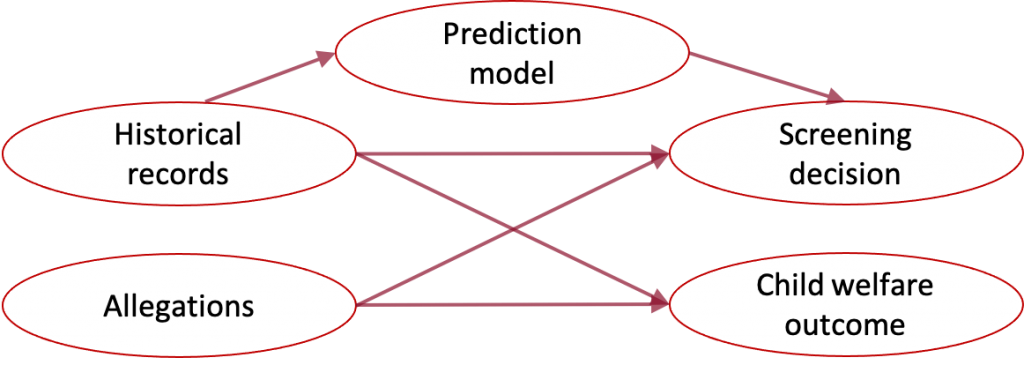
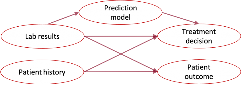
Figure 1. Due to feasibility or ethical requirements, a prediction model may only access a subset of the confounding factors that affect both the decision and outcome. We propose a procedure for learning valid counterfactual predictions in this setting.
In machine learning, we often want to predict the likelihood of an outcome if we take a proposed decision or action. A healthcare setting, for instance, may require predicting whether a patient will be re-admitted to the hospital if the patient receives a particular treatment. In the child welfare setting, a social worker needs to assess the likelihood of adverse outcomes if the agency offers family services. In such settings, algorithmic predictions can be used to help decision-makers. Since the prediction target depends on a particular decision (e.g., the particular medical treatment, or offering family services), we refer to these predictions as counterfactual.
In general, for valid counterfactual inference, we need to measure all factors that affect both the decision and the outcome of interest. However, we may not want to use all such factors in our prediction model. Some factors such as race or gender may be too sensitive to use for prediction. Some factors may be too complex to use when model interpretability is desired, or some factors may be difficult to measure at prediction time.
Child welfare example: The child welfare screening task requires a social worker to decide which calls to the child welfare hotline should be investigated. In jurisdictions such as Allegheny County, the social worker makes their decision based on allegations in the call and historical information about individuals associated with the call, such as their prior child welfare interaction and criminal justice history. Both the call allegations and historical information may contain factors that affect both the decision and future child outcomes, but the child welfare agency may be unable to parse and preprocess call information in real-time for use in a prediction system. The social worker would still benefit from a prediction that summarizes the risk based on historical information. Therefore, the goal is a prediction based on a subset of the confounding factors.
Healthcare example: Healthcare providers may make decisions based on the patient’s history as well as lab results and diagnostic tests, but the patient’s health record may not be in a form that can be easily input to a prediction algorithm.
How can we make counterfactual predictions using only a subset of confounding factors?
We propose a method for using offline data to build a prediction model that only requires access to the available subset of confounders at prediction time. Offline data is an important part of the solution because if we know nothing about the unmeasured confounders, then in general we cannot make progress. Fortunately, in our settings of interest, it is often possible to obtain an offline dataset that contains measurements of the full set of confounders as well as the outcome of interest and historical decision.
What is “runtime confounding?”
Runtime confounding occurs when all confounding factors are recorded in the training data, but the prediction model cannot use all confounding factors as features due to sensitivity, interpretability, or feasibility requirements. As examples,
- It may not be possible to measure factors efficiently enough for use in the prediction model but it is possible to measure factors offline with sufficient processing time. Child welfare agencies typically do record call allegations for offline processing.
- It may be undesirable to use some factors that are too sensitive or too complex for use in a prediction model.
Formally, let (V in mathbb{R}^{d_v}) denote the vector of factors available for prediction and (Z in mathbb{R}^{d_z}) denote the vector of confounding factors unavailable for prediction (but available in the training data). Given (V), our goal is to predict an outcome under a proposed decision; we wish to predict the potential outcome (Y^{A=a}) that we would observe under decision (a).
Prediction target: $$nu(v) := mathbb{E}[Y^{A=a} mid V = v] .$$ In order to estimate this hypothetical counterfactual quantity, we need assumptions that enable us to identify this quantity with observable data. We require three assumptions that are standard in causal inference:
Assumption 1: The decision assigned to one unit does not affect the potential outcomes of another unit.
Assumption 2: All units have some non-zero probability of receiving decision (a) (the decision of interest for prediction).
Assumption 3: (V,Z) describe all factors that jointly affect the decision and outcome.
These assumptions enable us to identify our target estimand as $$nu(v) = mathbb{E}[ mathbb{E}[Y mid A = a, V = v, Z =z] mid V =v].$$
This suggests that we can estimate an outcome model (mu(v,z) := mathbb{E}[Y mid A = a, V = v, Z =z]) and then regress the outcome model estimates on (V).
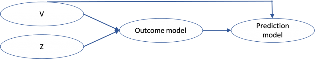
The simple plug-in (PL) approach:
- Estimate the outcome model (mu(v,z)) by regressing (Y sim V, Zmid A = a). Use this model to construct pseudo-outcomes (hat{mu}(V,Z)) for each case in our training data.
- Regress (hat{mu}(V,Z) sim V) to yield a prediction model that only requires knowledge of (V).
How does the PL approach perform?
- Yields valid counterfactual predictions under our three causal assumptions.
- Not optimal: Consider the setting in which (d_z >> d_v), for instance, in the child welfare setting where (Z) corresponds to the natural language in the hotline call. The PL approach requires us to efficiently estimate a more challenging high-dimensional target (mathbb{E}[Y mid A = a, V = v, Z =z]) when our target is a lower-dimensional quantity (nu(V)).
We can better take advantage of the lower-dimensional structure of our target estimand using doubly-robust techniques, which are popular in causal inference because they give us two chances to get our estimation right.
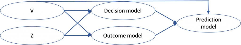
Our proposed doubly-robust (DR) approach
In addition to estimating the outcome model like the PL approach, a doubly-robust approach also estimates a decision model (pi(v,z) := mathbb{E}[mathbb{I}{A=a} mid V = v, Z =z]), which is known as the propensity model in causal inference. This is particularly helpful in settings where it is easier to estimate the decision model than the outcome model.
We propose a doubly-robust (DR) approach that also involves two stages:
- Regress (Y sim V, Zmid A = a) to yield outcome model (hat{mu}(v,z)). Regress (mathbb{I}{A=a} sim V, Z) to yield decision model (hat{pi}(v,z)).
- Regress $$frac{mathbb{I}{A=a}}{hat{pi}(V,Z)}(Y – hat{mu}(V,Z)) + hat{mu}(V,Z) sim V.$$
When does the DR approach perform well?
- When we can build either a very good outcome model or a very good decision model
- If both the decision model and outcome model are somewhat good
The DR approach can achieve oracle optimality–that is, it achieves the same regression error (up to constants) as an oracle with access to the true potential outcomes (Y^a).
We can see this by bounding the error of our method (hat{nu}) with the sum of the oracle error and a product of error terms on the outcome and decision models:
begin{align}
mathbb{E}[(hat{nu}(v) – nu(v))^2] ≲
& mathbb{E}[(tilde{nu}(v) – nu(v))^2] + \
& mathbb{E}[(hat{pi}(V,Z) -pi(V,Z))^2 mid V = v]mathbb{E}[(hat{mu}(V,Z) -mu(V,Z))^2 mid V = v].
end{align}
where (tilde{nu}(v)) denotes the function we would get in our second-stage estimation if we had oracle access to (Y^a).
So as long as we can estimate the outcome and decision models such that their product of errors is smaller than the oracle error, then the DR approach is oracle-efficient. This result holds for any regression method, assuming that we have used sample-splitting to learn (hat{nu}), (hat{mu}), and (hat{pi}).
While the DR approach has this desirable theoretical guarantee, in practice is it possible that the PL approach may perform better depending on the dimensionality of the problem.
How do I know which method I should use?
To determine which method will work best in a given setting, we provide an evaluation procedure that can be applied to any prediction method to estimate its mean-squared error. Under our three causal assumptions, the prediction error of a model (hat{nu}) is identified as
$$mathbb{E}[(Y^a – hat{nu}(V))^2] = mathbb{E}[mathbb{E}[(Y-hat{nu}(V)^2 mid V, Z, A = a]].$$
Defining the error regression (eta(v,z) = mathbb{E}[(Y-hat{nu}(V))^2 mid V = v, Z =a, A = a] ), we propose the following doubly-robust estimator for the MSE on a validation sample of (n) cases:
$$frac{1}{n} sum_{i=1}^n left[ frac{mathbb{I}{A_i = a }}{hat{pi}(V_i, Z_i)} left( (Y_i -hat{nu}(V_i))^2 – hat{eta}(V_i, Z_i) right) + hat{eta}(V_i, Z_i) right] .$$
Under mild assumptions, this estimator is (sqrt{n}) consistent, enabling us to get error estimates with confidence intervals.
DR achieves lowest MSE in synthetic experiments
We perform simulations on synthetic data to show how the level of confounding and dimensionalities of (V) and (Z) determine which method performs best. Synthetic experiments enable us to evaluate the methods on the ground-truth counterfactual outcomes. We compare the PL and DR approaches to a biased single-stage approach that estimates (mathbb{E}[Y mid V, A =a]), which we refer to as the treatment-conditional regression (TCR) approach.
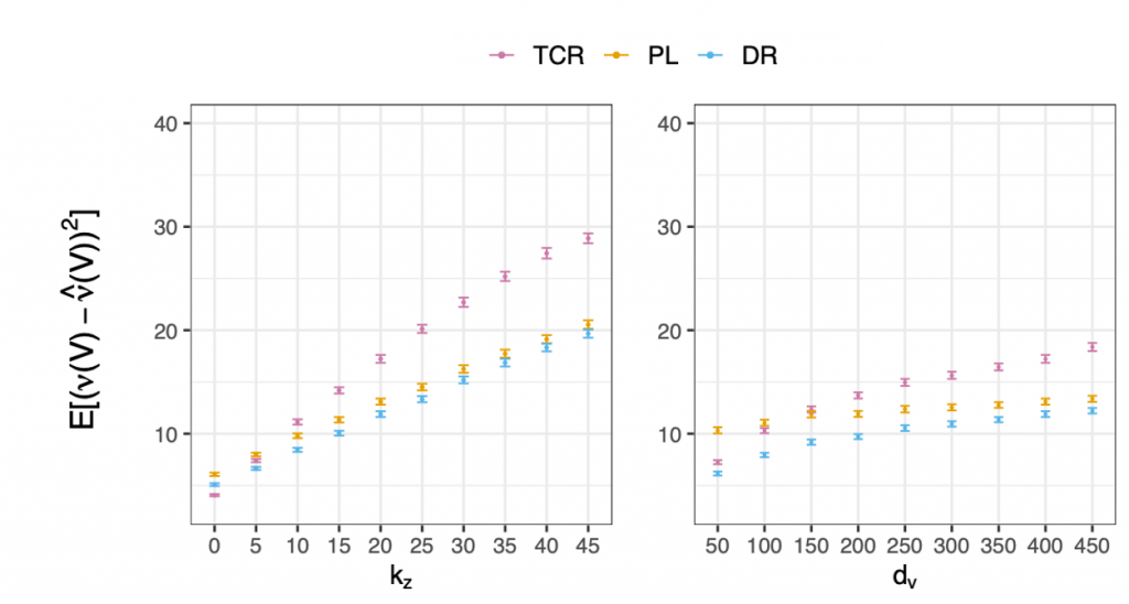
In the left-hand panel above, we compare the method as we vary the amount of confounding. When there is no confounding ((k_z = 0)), the TCR approach performs best as expected. Under no confounding, the TCR approach is no longer biased and efficiently estimates the target of interest in one stage. However, as we increase the level of confounding, the TCR performance degrades faster than the PL and DR methods. The DR method performs best under any non-zero level of confounding.
The right-hand panel compares the methods as we vary the dimensionality of our predictors. We hold the total dimensionality of ((V, Z)) fixed at (500) (so (d_z = 500 – d_v)). The DR approach performs best across the board, and the TCR approach performs well when the dimensionality is low because TCR avoids the high-dimensional second stage regression. However, this advantage disappears as (d_v) increases. The gap between the PL and DR methods is largest for low (d_v) because the DR method is able to take advantage of the lower dimensional target. At high (d_v) the PL error approaches the DR error.
DR is comparable to PL in a real-world task
We compare the methods on a real-world child welfare screening task where the goal is to predict the likelihood that a case will require services under the decision “screened in for investigation” using historical information as predictors and controlling for confounders that are sensitive (race) and hard to process (the allegations in the call). Our dataset consists of over 30,000 calls to the child welfare hotline in Allegheny County, PA. We evaluate the methods using our proposed real-world evaluation procedure since we do not have access to the ground-truth outcomes for cases that were not screened in for investigation.
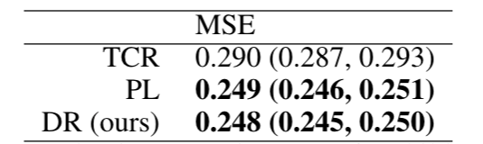
We find that the DR and PL approach perform comparably on this task, both outperforming the TCR method.
Recap
- Runtime confounding arises when it is undesirable or impermissible to use some confounding factors in the prediction model.
- We propose a generic procedure to build counterfactual predictions when the factors are available in offline training data.
- In theory, our approach is provably efficient in the oracle sense
- In practice, we recommend building the DR, PL, and TCR approaches and using our proposed evaluation scheme to choose the best performing model.
- Our full paper is available in the Proceedings of NeurIPS 2020.