Businesses can lose billions of dollars each year due to malicious users and fraudulent transactions. As more and more business operations move online, fraud and abuses in online systems are also on the rise. To combat online fraud, many businesses have been using rule-based fraud detection systems.
However, traditional fraud detection systems rely on a set of rules and filters hand-crafted by human specialists. The filters can often be brittle and the rules may not capture the full spectrum of fraudulent signals. Furthermore, while fraudulent behaviors are ever-evolving, the static nature of predefined rules and filters makes it difficult to maintain and improve traditional fraud detection systems effectively.
In this post, we show you how to build a dynamic, self-improving, and maintainable credit card fraud detection system with machine learning (ML) using Amazon SageMaker.
Alternatively, if you’re looking for a fully managed service to build customized fraud detection models without writing code, we recommend checking out Amazon Fraud Detector. Amazon Fraud Detector enables customers with no ML experience to automate building fraud detection models customized for their data, leveraging more than 20 years of fraud detection expertise from AWS and Amazon.com.
Solution overview
This solution builds the core of a credit card fraud detection system using SageMaker. We start by training an unsupervised anomaly detection model using the algorithm Random Cut Forest (RCF). Then we train two supervised classification models using the algorithm XGBoost, one as a baseline model and the other for making predictions, using different strategies to address the extreme class imbalance in data. Lastly, we train an optimal XGBoost model with hyperparameter optimization (HPO) to further improve the model performance.
For the sample dataset, we use the public, anonymized credit card transactions dataset that was originally released as part of a research collaboration of Worldline and the Machine Learning Group of ULB (Université Libre de Bruxelles). In the walkthrough, we also discuss how you can customize the solution to use your own data.
The outputs of the solution are as follows:
- An unsupervised SageMaker RCF model. The model outputs an anomaly score for each transaction. A low score value indicates that the transaction is considered normal (non-fraudulent). A high value indicates that the transaction is fraudulent. The definitions of low and high depend on the application, but common practice suggests that scores beyond three standard deviations from the mean score are considered anomalous.
- A supervised SageMaker XGBoost model trained using its built-in weighting schema to address the highly unbalanced data issue.
- A supervised SageMaker XGBoost model trained using the Sythetic Minority Over-sampling Technique (SMOTE).
- A trained SageMaker XGBoost model with HPO.
- Predictions of the probability for each transaction being fraudulent. If the estimated probability of a transaction is over a threshold, it’s classified as fraudulent.
To demonstrate how you can use this solution in your existing business infrastructures, we also include an example of making REST API calls to the deployed model endpoint, using AWS Lambda to trigger both the RCF and XGBoost models.
The following diagram illustrates the solution architecture.

Prerequisites
To try out the solution in your own account, make sure that you have the following in place:
- You need an AWS account to use this solution. If you don’t have an account, you can sign up for one.
- The solution outlined in this post is part of Amazon SageMaker JumpStart. To run this SageMaker JumpStart 1P Solution and have the infrastructure deploy to your AWS account, you need to create an active Amazon SageMaker Studio instance (see Onboard to Amazon SageMaker Domain).
When the Studio instance is ready, you can launch Studio and access JumpStart. JumpStart solutions are not available in SageMaker notebook instances, and you can’t access them through SageMaker APIs or the AWS Command Line Interface (AWS CLI).
Launch the solution
To launch the solution, complete the following steps:
- Open JumpStart by using the JumpStart launcher in the Get Started section or by choosing the JumpStart icon in the left sidebar.
- Under Solutions, choose Detect Malicious Users and Transactions to open the solution in another Studio tab.

- On the solution tab, choose Launch to launch the solution.

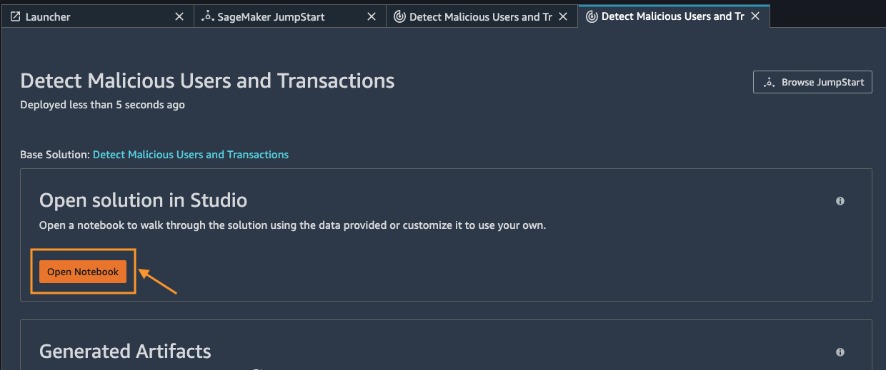
The solution resources are provisioned and another tab opens showing the deployment progress. When the deployment is finished, an Open Notebook button appears. - Choose Open Notebook to open the solution notebook in Studio.


Investigate and process the data
The default dataset contains only numerical features, because the original features have been transformed using Principal Component Analysis (PCA) to protect user privacy. As a result, the dataset contains 28 PCA components, V1–V28, and two features that haven’t been transformed, Amount and Time. Amount refers to the transaction amount, and Time is the seconds elapsed between any transaction in the data and the first transaction.
The Class column corresponds to whether or not a transaction is fraudulent.
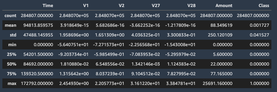
We can see that the majority is non-fraudulent, because out of the total 284,807 examples, only 492 (0.173%) are fraudulent. This is a case of extreme class imbalance, which is common in fraud detection scenarios.

We then prepare our data for loading and training. We split the data into a train set and a test set, using the former to train and the latter to evaluate the performance of our model. It’s important to split the data before applying any techniques to alleviate the class imbalance. Otherwise, we might leak information from the test set into the train set and hurt the model’s performance.
If you want to bring in your own training data, make sure that it’s tabular data in CSV format, upload the data to an Amazon Simple Storage Service (Amazon S3) bucket, and edit the S3 object path in the notebook code.

If your data includes categorical columns with non-numerical values, you need to one-hot encode these values (using, for example, sklearn’s OneHotEncoder) because the XGBoost algorithm only supports numerical data.
Train an unsupervised Random Cut Forest model
In a fraud detection scenario, we commonly have very few labeled examples, and labeling fraud can take a lot of time and effort. Therefore, we also want to extract information from the unlabeled data at hand. We do this using an anomaly detection algorithm, taking advantage of the high data imbalance that is common in fraud detection datasets.
Anomaly detection is a form of unsupervised learning where we try to identify anomalous examples based solely on their feature characteristics. Random Cut Forest is a state-of-the-art anomaly detection algorithm that is both accurate and scalable. With each data example, RCF associates an anomaly score.
We use the SageMaker built-in RCF algorithm to train an anomaly detection model on our training dataset, then make predictions on our test dataset.
First, we examine and plot the predicted anomaly scores for positive (fraudulent) and negative (non-fraudulent) examples separately, because the numbers of positive and negative examples differ significantly. We expect the positive (fraudulent) examples to have relatively high anomaly scores, and the negative (non-fraudulent) ones to have low anomaly scores. From the histograms, we can see the following patterns:
- Almost half of the positive examples (left histogram) have anomaly scores higher than 0.9, whereas most of the negative examples (right histogram) have anomaly scores lower than 0.85.
- The unsupervised learning algorithm RCF has limitations to identify fraudulent and non-fraudulent examples accurately. This is because no label information is used. We address this issue by collecting label information and using a supervised learning algorithm in later steps.

Then, we assume a more real-world scenario where we classify each test example as either positive (fraudulent) or negative (non-fraudulent) based on its anomaly score. We plot the score histogram for all test examples as follows, choosing a cutoff score of 1.0 (based on the pattern shown in the histogram) for classification. Specifically, if an example’s anomaly score is less than or equal to 1.0, it’s classified as negative (non-fraudulent). Otherwise, the example is classified as positive (fraudulent).

Lastly, we compare the classification result with the ground truth labels and compute the evaluation metrics. Because our dataset is imbalanced, we use the evaluation metrics balanced accuracy, Cohen’s Kappa score, F1 score, and ROC AUC, because they take into account the frequency of each class in the data. For all of these metrics, a larger value indicates a better predictive performance. Note that in this step we can’t compute the ROC AUC yet, because there is no estimated probability for positive and negative classes from the RCF model on each example. We compute this metric in later steps using supervised learning algorithms.
| . | RCF |
| Balanced accuracy | 0.560023 |
| Cohen’s Kappa | 0.003917 |
| F1 | 0.007082 |
| ROC AUC | – |
From this step, we can see that the unsupervised model can already achieve some separation between the classes, with higher anomaly scores correlated with fraudulent examples.
Train an XGBoost model with the built-in weighting schema
After we’ve gathered an adequate amount of labeled training data, we can use a supervised learning algorithm to discover relationships between the features and the classes. We choose the XGBoost algorithm because it has a proven track record, is highly scalable, and can deal with missing data. We need to handle the data imbalance this time, otherwise the majority class (the non-fraudulent, or negative examples) will dominate the learning.
We train and deploy our first supervised model using the SageMaker built-in XGBoost algorithm container. This is our baseline model. To handle the data imbalance, we use the hyperparameter scale_pos_weight, which scales the weights of the positive class examples against the negative class examples. Because the dataset is highly skewed, we set this hyperparameter to a conservative value: sqrt(num_nonfraud/num_fraud).
We train and deploy the model as follows:
- Retrieve the SageMaker XGBoost container URI.
- Set the hyperparameters we want to use for the model training, including the one we mentioned that handles data imbalance,
scale_pos_weight. - Create an XGBoost estimator and train it with our train dataset.
- Deploy the trained XGBoost model to a SageMaker managed endpoint.
- Evaluate this baseline model with our test dataset.
Then we evaluate our model with the same four metrics as mentioned in the last step. This time we can also calculate the ROC AUC metric.
| . | RCF | XGBoost |
| Balanced accuracy | 0.560023 | 0.847685 |
| Cohen’s Kappa | 0.003917 | 0.743801 |
| F1 | 0.007082 | 0.744186 |
| ROC AUC | – | 0.983515 |
We can see that a supervised learning method XGBoost with the weighting schema (using the hyperparameter scale_pos_weight) achieves significantly better performance than the unsupervised learning method RCF. There is still room to improve the performance, however. In particular, raising the Cohen’s Kappa score above 0.8 would be generally very favorable.
Apart from single-value metrics, it’s also useful to look at metrics that indicate performance per class. For example, the confusion matrix, per-class precision, recall, and F1-score can provide more information about our model’s performance.
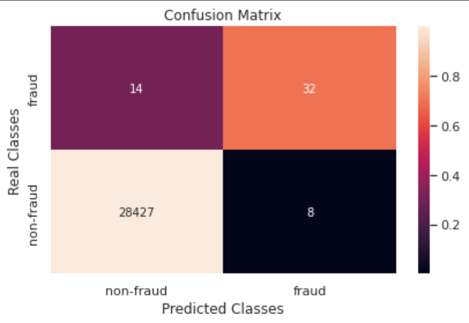
| . | precision | recall | f1-score | support |
| non-fraud | 1.00 | 1.00 | 1.00 | 28435 |
| fraud | 0.80 | 0.70 | 0.74 | 46 |
Keep sending test traffic to the endpoint via Lambda
To demonstrate how to use our models in a production system, we built a REST API with Amazon API Gateway and a Lambda function. When client applications send HTTP inference requests to the REST API, which triggers the Lambda function, which in turn invokes the RCF and XGBoost model endpoints and returns the predictions from the models. You can read the Lambda function code and monitor the invocations on the Lambda console.
We also created a Python script that makes HTTP inference requests to the REST API, with our test data as input data. To see how this was done, check the generate_endpoint_traffic.py file in the solution’s source code. The prediction outputs are logged to an S3 bucket through an Amazon Kinesis Data Firehose delivery stream. You can find the destination S3 bucket name on the Kinesis Data Firehose console, and check the prediction results in the S3 bucket.
Train an XGBoost model with the over-sampling technique SMOTE
Now that we have a baseline model using XGBoost, we can see if sampling techniques that are designed specifically for imbalanced problems can improve the performance of the model. We use Sythetic Minority Over-sampling (SMOTE), which oversamples the minority class by interpolating new data points between existing ones.
The steps are as follows:
- Use SMOTE to oversample the minority class (the fraudulent class) of our train dataset. SMOTE oversamples the minority class from about 0.17–50%. Note that this is a case of extreme oversampling of the minority class. An alternative would be to use a smaller resampling ratio, such as having one minority class sample for every
sqrt(non_fraud/fraud)majority sample, or using more advanced resampling techniques. For more over-sampling options, refer to Compare over-sampling samplers. - Define the hyperparameters for training the second XGBoost so that scale_pos_weight is removed and the other hyperparameters remain the same as when training the baseline XGBoost model. We don’t need to handle data imbalance with this hyperparameter anymore, because we’ve already done that with SMOTE.
- Train the second XGBoost model with the new hyperparameters on the SMOTE processed train dataset.
- Deploy the new XGBoost model to a SageMaker managed endpoint.
- Evaluate the new model with the test dataset.
When evaluating the new model, we can see that with SMOTE, XGBoost achieves a better performance on balanced accuracy, but not on Cohen’s Kappa and F1 scores. The reason for this is that SMOTE has oversampled the fraud class so much that it’s increased its overlap in feature space with the non-fraud cases. Because Cohen’s Kappa gives more weight to false positives than balanced accuracy does, the metric drops significantly, as does the precision and F1 score for fraud cases.
| . | RCF | XGBoost | XGBoost SMOTE |
| Balanced accuracy | 0.560023 | 0.847685 | 0.912657 |
| Cohen’s Kappa | 0.003917 | 0.743801 | 0.716463 |
| F1 | 0.007082 | 0.744186 | 0.716981 |
| ROC AUC | – | 0.983515 | 0.967497 |
However, we can bring back the balance between metrics by adjusting the classification threshold. So far, we’ve been using 0.5 as the threshold to label whether or not a data point is fraudulent. After experimenting different thresholds from 0.1–0.9, we can see that Cohen’s Kappa keeps increasing along with the threshold, without a significant loss in balanced accuracy.
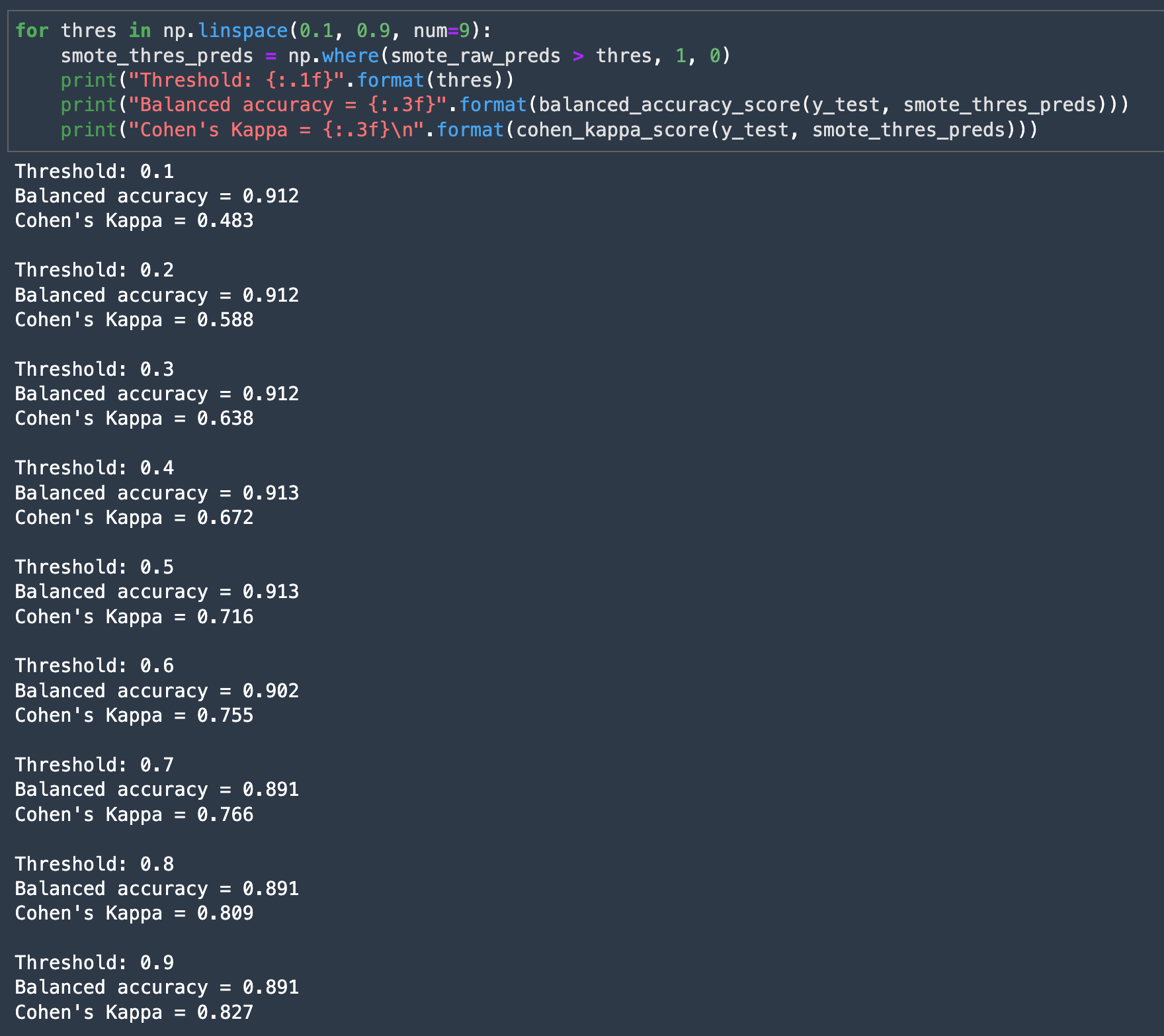
This adds a useful calibration to our model. We can use a low threshold if not missing any fraudulent cases (false negatives) is our priority, or we can increase the threshold to minimize the number of false positives.
Train an optimal XGBoost model with HPO
In this step, we demonstrate how to improve model performance by training our third XGBoost model with hyperparameter optimization. When building complex ML systems, manually exploring all possible combinations of hyperparameter values is impractical. The HPO feature in SageMaker can accelerate your productivity by trying many variations of a model on your behalf. It automatically looks for the best model by focusing on the most promising combinations of hyperparameter values within the ranges that you specify.
The HPO process needs a validation dataset, so we first further split our training data into training and validation datasets using stratified sampling. To tackle the data imbalance problem, we use XGBoost’s weighting schema again, setting the scale_pos_weight hyperparameter to sqrt(num_nonfraud/num_fraud).
We create an XGBoost estimator using the SageMaker built-in XGBoost algorithm container, and specify the objective evaluation metric and the hyperparameter ranges within which we’d like to experiment. With these we then create a HyperparameterTuner and kick off the HPO tuning job, which trains multiple models in parallel, looking for optimal hyperparameter combinations.
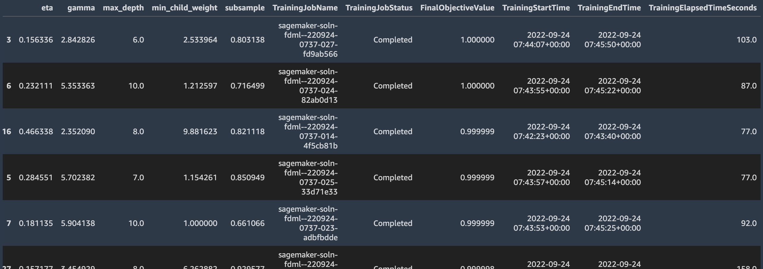
When the tuning job is complete, we can see its analytics report and inspect each model’s hyperparameters, training job information, and its performance against the objective evaluation metric.
Then we deploy the best model and evaluate it with our test dataset.
Evaluate and compare all model performance on the same test data
Now we have the evaluation results from all four models: RCF, XGBoost baseline, XGBoost with SMOTE, and XGBoost with HPO. Let’s compare their performance.
| . | RCF | XGBoost | XGBoost with SMOTE | XGBoost with HPO |
| Balanced accuracy | 0.560023 | 0.847685 | 0.912657 | 0.902156 |
| Cohen’s Kappa | 0.003917 | 0.743801 | 0.716463 | 0.880778 |
| F1 | 0.007082 | 0.744186 | 0.716981 | 0.880952 |
| ROC AUC | – | 0.983515 | 0.967497 | 0.981564 |
We can see that XGBoost with HPO achieves even better performance than that with the SMOTE method. In particular, Cohen’s Kappa scores and F1 are over 0.8, indicating an optimal model performance.
Clean up
When you’re finished with this solution, make sure that you delete all unwanted AWS resources to avoid incurring unintended charges. In the Delete solution section on your solution tab, choose Delete all resources to delete resources automatically created when launching this solution.

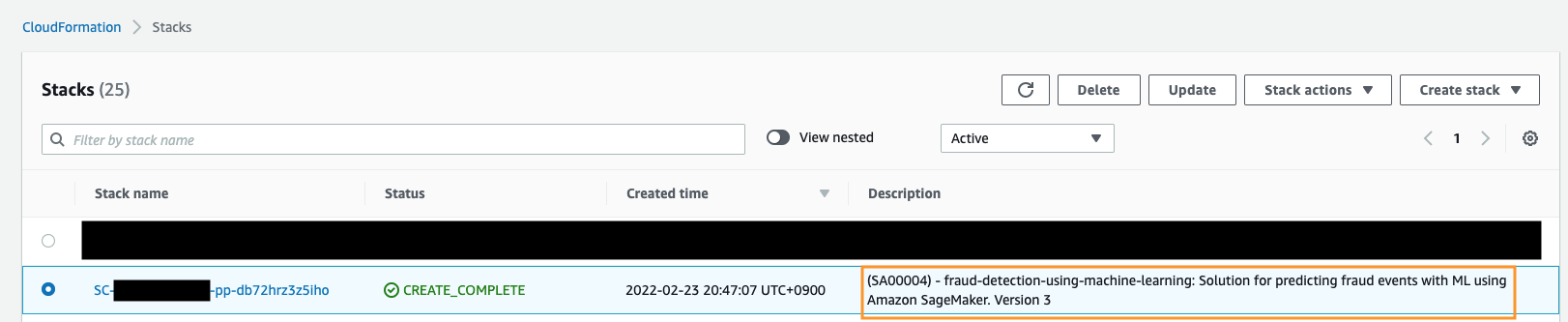
Alternatively, you can use AWS CloudFormation to delete all standard resources automatically created by the solution and notebook. To use this approach, on the AWS CloudFormation console, find the CloudFormation stack whose description contains fraud-detection-using-machine-learning, and delete it. This is a parent stack, and choosing to delete this stack will automatically delete the nested stacks.
With either approach, you still need to manually delete any extra resources that you may have created in this notebook. Some examples include extra S3 buckets (in addition to the solution’s default bucket), extra SageMaker endpoints (using a custom name), and extra Amazon Elastic Container Registry (Amazon ECR) repositories.
Conclusion
In this post, we showed you how to build the core of a dynamic, self-improving, and maintainable credit card fraud detection system using ML with SageMaker. We built, trained, and deployed an unsupervised RCF anomaly detection model, a supervised XGBoost model as the baseline, another supervised XGBoost model with SMOTE to tackle the data imbalance problem, and a final XGBoost model optimized with HPO. We discussed how to handle data imbalance and use your own data in the solution. We also included an example REST API implementation with API Gateway and Lambda to demonstrate how to use the system in your existing business infrastructure.
To try it out yourself, open SageMaker Studio and launch the JumpStart solution. To learn more about the solution, check out its GitHub repository.
About the Authors
 Xiaoli Shen is a Solutions Architect and Machine Learning Technical Field Community (TFC) member at Amazon Web Services. She’s focused on helping customers architecting on the cloud and leveraging AWS services to derive business value. Prior to joining AWS, she was a tech lead and senior full-stack engineer building data-intensive distributed systems on the cloud.
 Dr. Xin Huang is an Applied Scientist for Amazon SageMaker JumpStart and Amazon SageMaker built-in algorithms. He focuses on developing scalable machine learning algorithms. His research interests are in the area of natural language processing, explainable deep learning on tabular data, and robust analysis of non-parametric space-time clustering. He has published many papers in ACL, ICDM, KDD conferences, and Royal Statistical Society: Series A journal.
 Vedant Jain is a Sr. AI/ML Specialist Solutions Architect, helping customers derive value out of the Machine Learning ecosystem at AWS. Prior to joining AWS, Vedant has held ML/Data Science Specialty positions at various companies such as Databricks, Hortonworks (now Cloudera) & JP Morgan Chase. Outside of his work, Vedant is passionate about making music, using Science to lead a meaningful life & exploring delicious vegetarian cuisine from around the world.