Introduction
PyTorch 2.0 (PT2) offers a compiled execution mode which rewrites Python bytecode to extract sequences of PyTorch operations, translating them into a Graph IR. The IR is then just-in-time compiled through a customizable back end, improving training performance without user interference. Often, production models may go through multiple stages of optimization/lowering to hit performance targets. Therefore, having a compiled mode is desirable as it can separate the work of improving model performance from direct modification of the PyTorch model implementation. Thus, the compiled mode becomes more important, enabling Pytorch users to enhance model performance without modifying the PyTorch code implementation. This feature is particularly valuable for optimizing complex models, including large-scale and production-ready ones.
In our previous blog post , we outlined how heuristic model transformation rules are employed to optimize intricate production models. While these rules enabled substantial performance gains for some pilot models, they lacked universal adaptability; they don’t consistently perform well across different models or sometimes even within different sections of a single model.
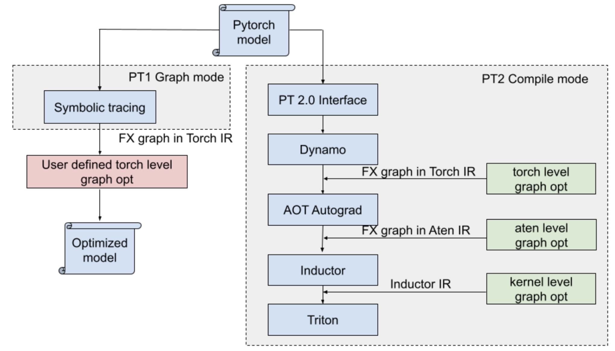
Fig. 1: PT1 Graph mode vs PT2 Compile mode.
In this blog post, we propose a more generalized model transformation solution, serving as a plugin to the PT2 compiler as shown in Fig.1 which is more general, performant and user-friendly, bringing performance improvements to both model training and inference without manual efforts. As illustrated in Fig.2, by incorporating the previously user-defined transformations into the compiler, we have streamlined the production stack. These changes bring advantages to a broader range of PyTorch models, extending beyond just Meta models, which has already been incorporated in PT2 and is ready for use to benefit all Pytorch models.
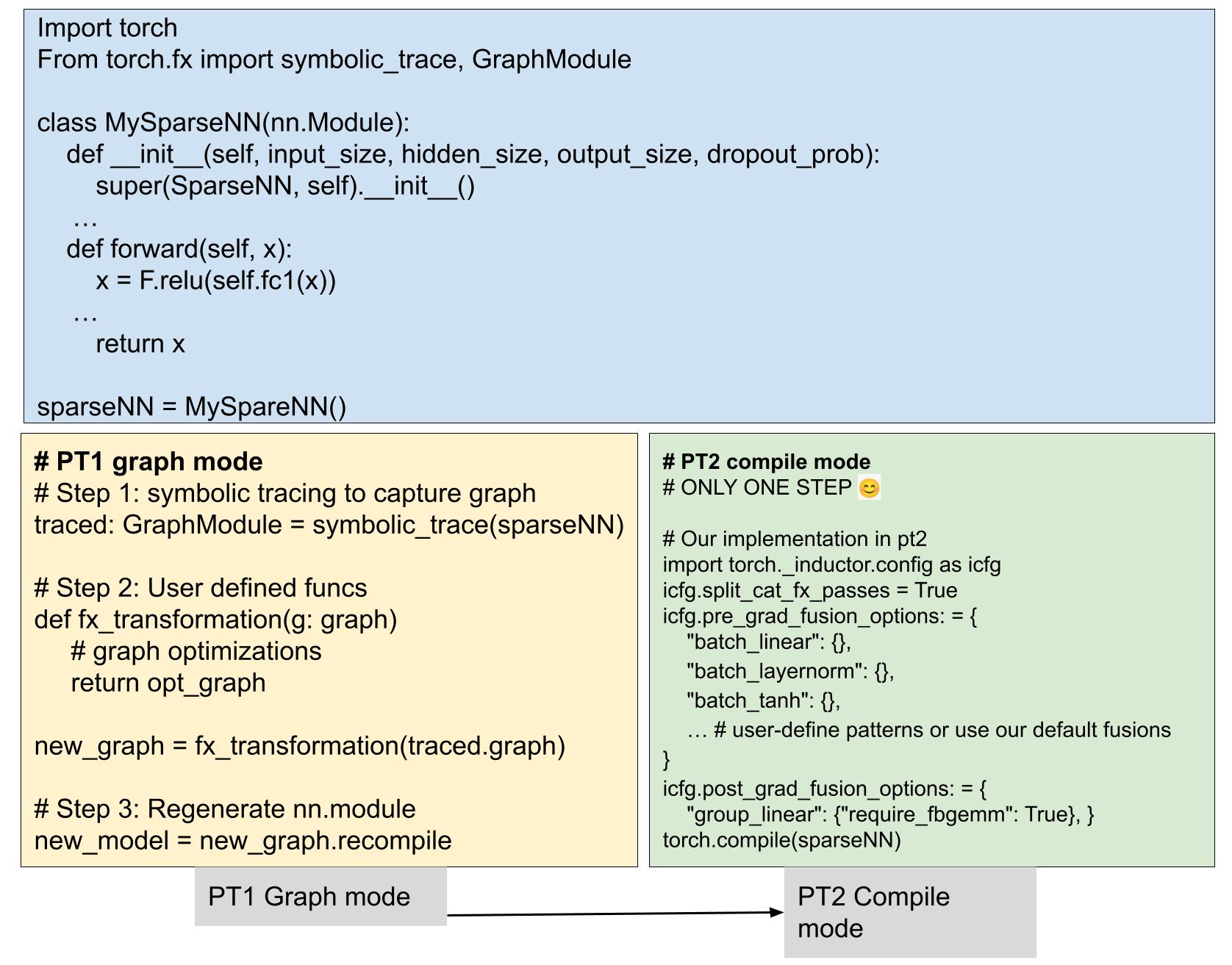
Fig. 2: Simplified stack with PT2 compile mode.
Guiding Principle: Atomic Rules
Traditionally, people might use predefined heuristic rules to replace a model subgraph with another more performant subgraph toreduce launch overhead, minimize memory bw, and fully occupy SMs. However, this approach doesn’t scale well as it is hard to craft a set of rules that fits all models perfectly.
Instead of grappling with bulky, complex rules, we can actually break them down into smaller, more digestible pieces – what we call ‘atomic rules’. These tiny powerhouses of efficiency target the transformation of individual operators, to conduct one step of the fusion/transformation. This makes them easy to handle and apply, offering a straightforward path to optimizing models. So, with these atomic rules in hand, optimizing any model for top-tier performance becomes a breeze!
We will walk through some simple examples to demonstrate how we use a chain of atomic rules to replace complicated heuristic rules.
Case 1: Horizontal fusion of computation chains started with accesses to embedding tables
Horizontal fusion means fusing parallel operators into one so as to reduce the number of kernels to be launched and improve performance. In our previous blog (Section 3.2), we described model transformations that fused layernorm and activation functions after embedding bags, as shown in the figure provided. However, this method, had limitations:
- It only worked with layernorm and activation functions after embedding.
- It was restricted to models with specific architecture rules, causing various issues in our production stack, including parameter changes and inference disruptions.
To improve, we can use three atomic rules as shown in Fig.3 to replace the complicated heuristic rule:
- Fuse layernorms that follow the same split nodes horizontally.
- Then, fuse tanh functions following the same split nodes horizontally.
- Lastly, fuse vertical split-cat nodes.
These atomic rules offer a clean and streamlined way for model simplification and optimization.
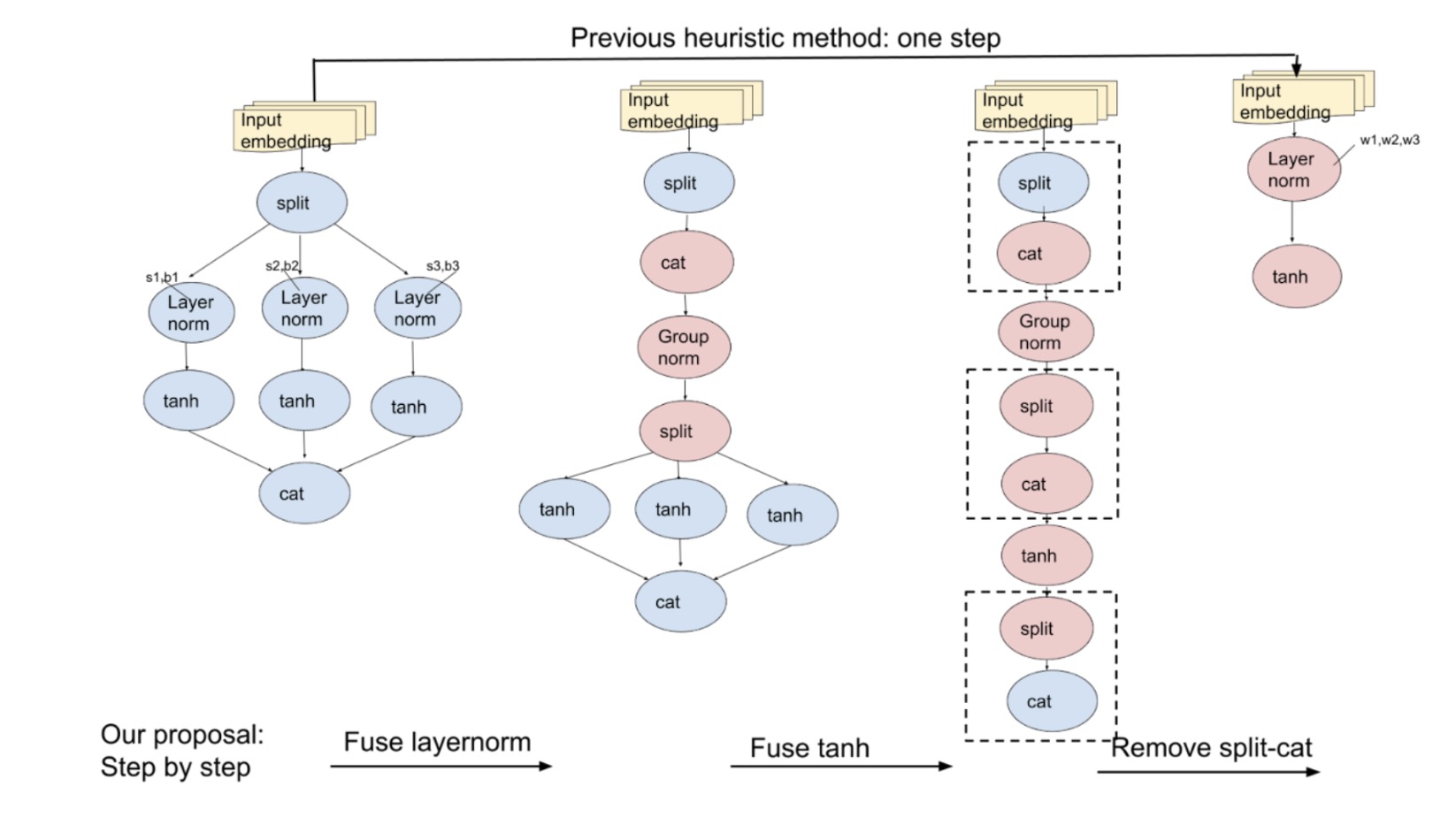
Fig. 3: Before, we optimized the model in one go by replacing subgraphs. Now, with atomic rules, we optimize step-by-step, covering more cases.
Case 2: Fuse horizontal MLP
MLPs (Multilayer Perceptrons) are fundamental components of deep neural networks, often consisting of linear, normalization, and activation functions. In complex models, there’s often a need to fuse many horizontal MLPs. Traditional methods find and replace parallel MLPs with a fused module as shown in Fig.4, but this isn’t always straightforward. Some models might not have normalization, or they might use different activation functions, making it hard to apply a one-size-fits-all rule.
This is where our atomic rules come in handy. These simplified rules target individual operators one at a time, making the process easier and more manageable. We use the following atomic rules for horizontal MLP fusion:
- Fusing horizontal linear operators
- Fusing horizontal layernorms.
- Fusing horizontal activation functions.
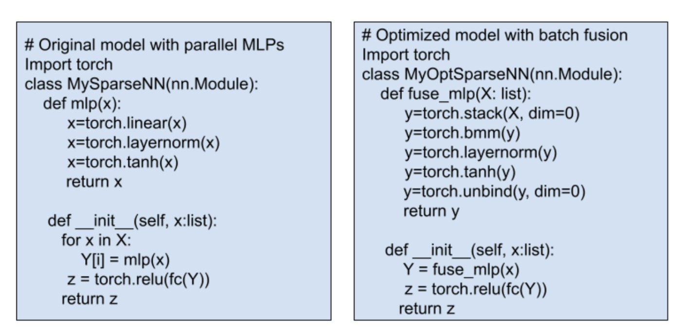
Fig. 4: Pseudocode for fusing MLP. Traditional optimizations need manual Python code changes.
The beauty of these rules is that they’re not limited to one case. They can be applied broadly. Since PyTorch models are built with torch operators, focusing on a smaller set of operators simplifies the process. This approach is not only more manageable but also more general compared to writing a specific large pattern replacement rule, making it easier to optimize various models efficiently.
Compile-time Graph Search
Our principle is to use chained atomic rules to replace heuristic rules. While this approach covers a wider range of cases, it does entail a longer time for graph search and pattern matching. The next question is: how can we minimize compilation time while performing compile-time graph searches efficiently?
We design a two-step greedy algorithm as illustrated in Fig. 5. The first step in this process is to identify the target nodes, which we follow certain rules, e.g., identifying all linear operations with the same input shapes. Once identified, we use a Breadth-First Search (BFS) strategy to separate these nodes into different sets, so that nodes within a set don’t have data dependency. The nodes within each of these sets are independent and can be fused horizontally.
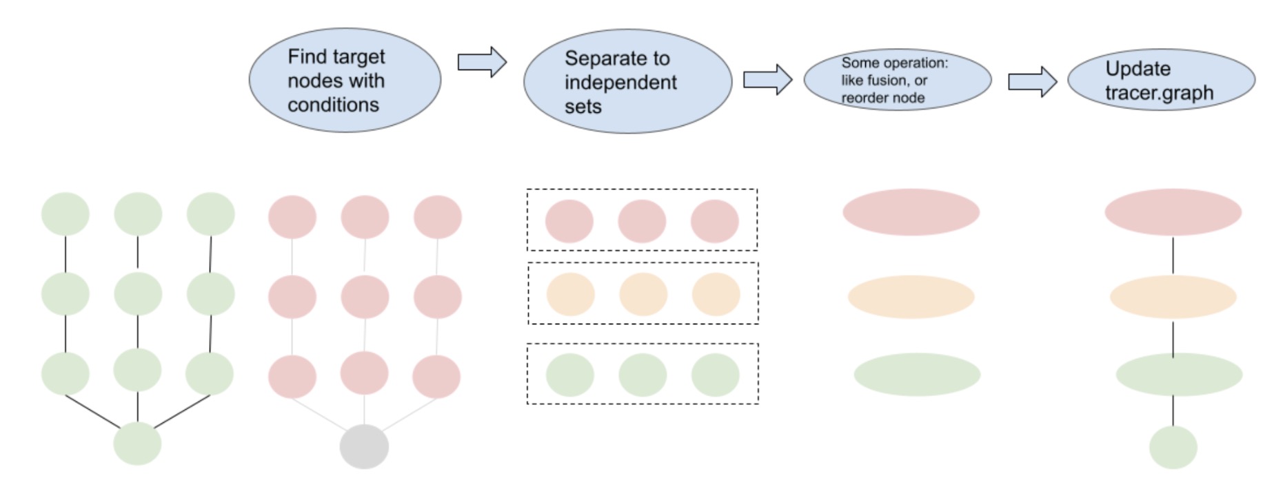
Fig. 5: Process of model transformation with graph IR.
With our approach, the search time is roughly 60 seconds for one of our largest internal models. It is manageable for on-the-fly tasks and
In the End
In our tests with internal ranking models, we observed approximately 5% to 15% training performance improvement across five models on top of the performance gain brought by torch.compile. We have enabled the optimization in PT2 compiler stack and landed it as default when users choose Inductor as the backend (config). We expect our generalized transformation approach could benefit models beyond Meta, and look forward to more discussion and improvement through this compiler level transformation framework.
Acknowledgements
Many thanks to Mark Saroufim, Gregory Chanan, Adnan Aziz, and Rocky Liu for their detailed and insightful reviews.