In TorchVision v0.9, we released a series of new mobile-friendly models that can be used for Classification, Object Detection and Semantic Segmentation. In this article, we will dig deep into the code of the models, share notable implementation details, explain how we configured and trained them, and highlight important tradeoffs we made during their tuning. Our goal is to disclose technical details that typically remain undocumented in the original papers and repos of the models.
Network Architecture
The implementation of the MobileNetV3 architecture follows closely the original paper. It is customizable and offers different configurations for building Classification, Object Detection and Semantic Segmentation backbones. It was designed to follow a similar structure to MobileNetV2 and the two share common building blocks.
Off-the-shelf, we offer the two variants described on the paper: the Large and the Small. Both are constructed using the same code with the only difference being their configuration which describes the number of blocks, their sizes, their activation functions etc.
Configuration parameters
Even though one can write a custom InvertedResidual setting and pass it to the MobileNetV3 class directly, for the majority of applications we can adapt the existing configs by passing parameters to the model building methods. Some of the key configuration parameters are the following:
-
The
width_multparameter is a multiplier that affects the number of channels of the model. The default value is 1 and by increasing or decreasing it one can change the number of filters of all convolutions, including the ones of the first and last layers. The implementation ensures that the number of filters is always a multiple of 8. This is a hardware optimization trick which allows for faster vectorization of operations. -
The
reduced_tailparameter halves the number of channels on the last blocks of the network. This version is used by some Object Detection and Semantic Segmentation models. It’s a speed optimization which is described on the MobileNetV3 paper and reportedly leads to a 15% latency reduction without a significant negative effect on accuracy. -
The
dilatedparameter affects the last 3 InvertedResidual blocks of the model and turns their normal depthwise Convolutions to Atrous Convolutions. This is used to control the output stride of these blocks and has a significant positive effect on the accuracy of Semantic Segmentation models.
Implementation details
Below we provide additional information on some notable implementation details of the architecture.
The MobileNetV3 class is responsible for building a network out of the provided configuration. Here are some implementation details of the class:
-
The last convolution block expands the output of the last InvertedResidual block by a factor of 6. The implementation is aligned with the Large and Small configurations described on the paper and can adapt to different values of the multiplier parameter.
-
Similarly to other models such as MobileNetV2, a dropout layer is placed just before the final Linear layer of the classifier.
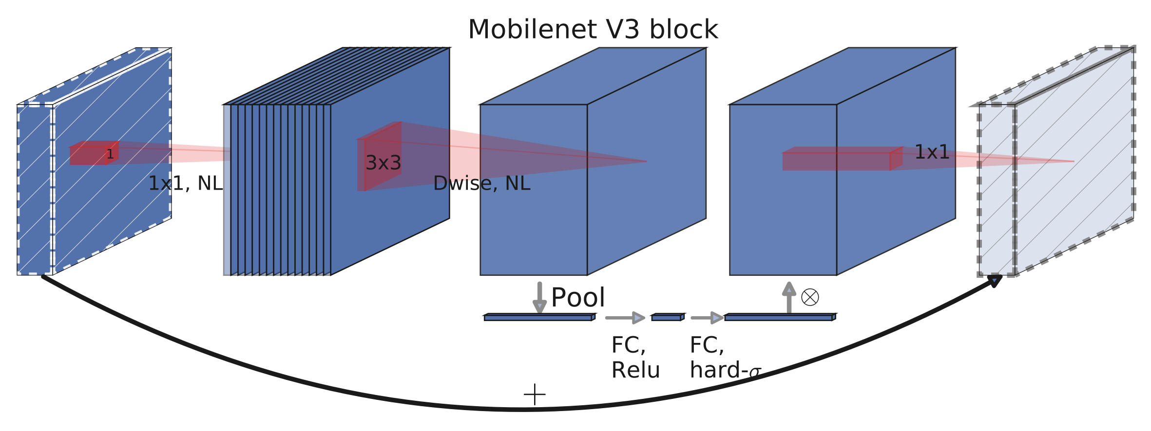
The InvertedResidual class is the main building block of the network. Here are some notable implementation details of the block along with its visualization which comes from Figure 4 of the paper:
-
There is no expansion step if the input channels and the expanded channels are the same. This happens on the first convolution block of the network.
-
There is always a projection step even when the expanded channels are the same as the output channels.
-
The activation method of the depthwise block is placed before the Squeeze-and-Excite layer as this improves marginally the accuracy.
Classification
In this section we provide benchmarks of the pre-trained models and details on how they were configured, trained and quantized.
Benchmarks
Here is how to initialize the pre-trained models:
large = torchvision.models.mobilenet_v3_large(pretrained=True, width_mult=1.0,  reduced_tail=False, dilated=False)
small = torchvision.models.mobilenet_v3_small(pretrained=True)
quantized = torchvision.models.quantization.mobilenet_v3_large(pretrained=True)
Below we have the detailed benchmarks between new and selected previous models. As we can see MobileNetV3-Large is a viable replacement of ResNet50 for users who are willing to sacrifice a bit of accuracy for a roughly 6x speed-up:
| Model | Acc@1 | Acc@5 | Inference on CPU (sec) | # Params (M) |
|---|---|---|---|---|
| MobileNetV3-Large | 74.042 | 91.340 | 0.0411 | 5.48 |
| MobileNetV3-Small | 67.668 | 87.402 | 0.0165 | 2.54 |
| Quantized MobileNetV3-Large | 73.004 | 90.858 | 0.0162 | 2.96 |
| MobileNetV2 | 71.880 | 90.290 | 0.0608 | 3.50 |
| ResNet50 | 76.150 | 92.870 | 0.2545 | 25.56 |
| ResNet18 | 69.760 | 89.080 | 0.1032 | 11.69 |
Note that the inference times are measured on CPU. They are not absolute benchmarks, but they allow for relative comparisons between models.
Training process
All pre-trained models are configured with a width multiplier of 1, have full tails, are non-dilated, and were fitted on ImageNet. Both the Large and Small variants were trained using the same hyper-parameters and scripts which can be found in our references folder. Below we provide details on the most notable aspects of the training process.
Achieving fast and stable training
Configuring RMSProp correctly was crucial to achieve fast training with numerical stability. The authors of the paper used TensorFlow in their experiments and in their runs they reported using quite high rmsprop_epsilon comparing to the default. Typically this hyper-parameter takes small values as it’s used to avoid zero denominators, but in this specific model choosing the right value seems important to avoid numerical instabilities in the loss.
Another important detail is that though PyTorch’s and TensorFlow’s RMSProp implementations typically behave similarly, there are a few differences with the most notable in our setup being how the epsilon hyperparameter is handled. More specifically, PyTorch adds the epsilon outside of the square root calculation while TensorFlow adds it inside. The result of this implementation detail is that one needs to adjust the epsilon value while porting the hyper parameter of the paper. A reasonable approximation can be taken with the formula PyTorch_eps = sqrt(TF_eps).
Increasing our accuracy by tuning hyperparameters & improving our training recipe
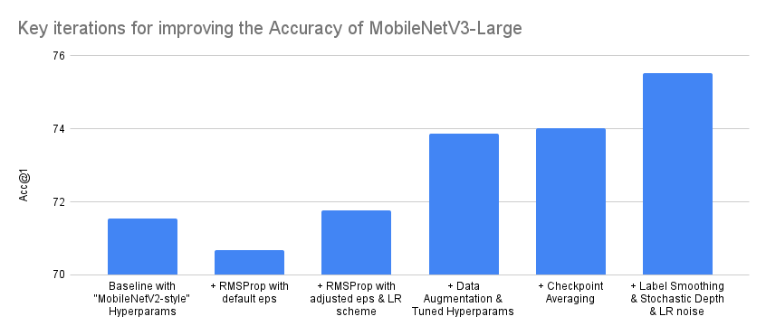
After configuring the optimizer to achieve fast and stable training, we turned into optimizing the accuracy of the model. There are a few techniques that helped us achieve this. First of all, to avoid overfitting we augmented out data using the AutoAugment algorithm, followed by RandomErasing. Additionally we tuned parameters such as the weight decay using cross validation. We also found beneficial to perform weight averaging across different epoch checkpoints after the end of the training. Finally, though not used in our published training recipe, we found that using Label Smoothing, Stochastic Depth and LR noise injection improve the overall accuracy by over 1.5 points.
The graph and table depict a simplified summary of the most important iterations for improving the accuracy of the MobileNetV3 Large variant. Note that the actual number of iterations done while training the model was significantly larger and that the progress in accuracy was not always monotonically increasing. Also note that the Y-axis of the graph starts from 70% instead from 0% to make the difference between iterations more visible:
| Iteration | Acc@1 | Acc@5 |
|---|---|---|
| Baseline with “MobileNetV2-style” Hyperparams | 71.542 | 90.068 |
| + RMSProp with default eps | 70.684 | 89.38 |
| + RMSProp with adjusted eps & LR scheme | 71.764 | 90.178 |
| + Data Augmentation & Tuned Hyperparams | 73.86 | 91.292 |
| + Checkpoint Averaging | 74.028 | 91.382 |
| + Label Smoothing & Stochastic Depth & LR noise | 75.536 | 92.368 |
Note that once we’ve achieved an acceptable accuracy, we verified the model performance on the hold-out test dataset which hasn’t been used before for training or hyper-parameter tuning. This process helps us detect overfitting and is always performed for all pre-trained models prior their release.
Quantization
We currently offer quantized weights for the QNNPACK backend of the MobileNetV3-Large variant which provides a speed-up of 2.5x. To quantize the model, Quantized Aware Training (QAT) was used. The hyper parameters and the scripts used to train the model can be found in our references folder.
Note that QAT allows us to model the effects of quantization and adjust the weights so that we can improve the model accuracy. This translates to an accuracy increase of 1.8 points comparing to simple post-training quantization:
| Quantization Status | Acc@1 | Acc@5 |
|---|---|---|
| Non-quantized | 74.042 | 91.340 |
| Quantized Aware Training | 73.004 | 90.858 |
| Post-training Quantization | 71.160 | 89.834 |
Object Detection
In this section, we will first provide benchmarks of the released models, and then discuss how the MobileNetV3-Large backbone was used in a Feature Pyramid Network along with the FasterRCNN detector to perform Object Detection. We will also explain how the network was trained and tuned alongside with any tradeoffs we had to make. We will not cover details about how it was used with SSDlite as this will be discussed on a future article.
Benchmarks
Here is how the models are initialized:
high_res = torchvision.models.detection.fasterrcnn_mobilenet_v3_large_fpn(pretrained=T low_res = torchvision.models.detection.fasterrcnn_mobilenet_v3_large_320_fpn(pretraine
Below are some benchmarks between new and selected previous models. As we can see the high resolution Faster R-CNN with MobileNetV3-Large FPN backbone seems a viable replacement of the equivalent ResNet50 model for those users who are willing to sacrifice few accuracy points for a 5x speed-up:
| Model | mAP | Inference on CPU (sec) | # Params (M) |
|---|---|---|---|
| Faster R-CNN MobileNetV3-Large FPN (High-Res) | 32.8 | 0.8409 | 19.39 |
| Faster R-CNN MobileNetV3-Large 320 FPN (Low-Res) | 22.8 | 0.1679 | 19.39 |
| Faster R-CNN ResNet-50 FPN | 37.0 | 4.1514 | 41.76 |
| RetinaNet ResNet-50 FPN | 36.4 | 4.8825 | 34.01 |
Implementation details
The Detector uses a FPN-style backbone which extracts features from different convolutions of the MobileNetV3 model. By default the pre-trained model uses the output of the 13th InvertedResidual block and the output of the Convolution prior to the pooling layer but the implementation supports using the outputs of more stages.
All feature maps extracted from the network have their output projected down to 256 channels by the FPN block as this greatly improves the speed of the network. These feature maps provided by the FPN backbone are used by the FasterRCNN detector to provide box and class predictions at different scales.
Training & Tuning process
We currently offer two pre-trained models capable of doing object detection at different resolutions. Both models were trained on the COCO dataset using the same hyper-parameters and scripts which can be found in our references folder.
The High Resolution detector was trained with images of 800-1333px, while the mobile-friendly Low Resolution detector was trained with images of 320-640px. The reason why we provide two separate sets of pre-trained weights is because training a detector directly on the smaller images leads to a 5 mAP increase in precision comparing to passing small images to the pre-trained high-res model. Both backbones were initialized with weights fitted on ImageNet and the 3 last stages of their weights where fined-tuned during the training process.
An additional speed optimization can be applied on the mobile-friendly model by tuning the RPN NMS thresholds. By sacrificing only 0.2 mAP of precision we were able to improve the CPU speed of the model by roughly 45%. The details of the optimization can be seen below:
| Tuning Status | mAP | Inference on CPU (sec) |
|---|---|---|
| Before | 23.0 | 0.2904 |
| After | 22.8 | 0.1679 |
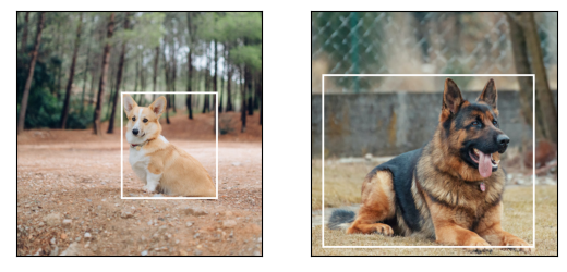
Below we provide some examples of visualizing the predictions of the Faster R-CNN MobileNetV3-Large FPN model:
Semantic Segmentation
In this section we will start by providing some benchmarks of the released pre-trained models. Then we will discuss how a MobileNetV3-Large backbone was combined with segmentation heads such as LR-ASPP, DeepLabV3 and the FCN to conduct Semantic Segmentation. We will also explain how the network was trained and propose a few optional optimization techniques for speed critical applications.
Benchmarks
This is how to initialize the pre-trained models:
lraspp = torchvision.models.segmentation.lraspp_mobilenet_v3_large(pretrained=True) deeplabv3 = torchvision.models.segmentation.deeplabv3_mobilenet_v3_large(pretrained=Tr
Below are the detailed benchmarks between new and selected existing models. As we can see, the DeepLabV3 with a MobileNetV3-Large backbone is a viable replacement of FCN with ResNet50 for the majority of applications as it achieves similar accuracy with a 8.5x speed-up. We also observe that the LR-ASPP network supersedes the equivalent FCN in all metrics:
| Model | mIoU | Global Pixel Acc | Inference on CPU (sec) | # Params (M) |
|---|---|---|---|---|
| LR-ASPP MobileNetV3-Large | 57.9 | 91.2 | 0.3278 | 3.22 |
| DeepLabV3 MobileNetV3-Large | 60.3 | 91.2 | 0.5869 | 11.03 |
| FCN MobileNetV3-Large (not released) | 57.8 | 90.9 | 0.3702 | 5.05 |
| DeepLabV3 ResNet50 | 66.4 | 92.4 | 6.3531 | 39.64 |
| FCN ResNet50 | 60.5 | 91.4 | 5.0146 | 32.96 |
Implementation details
In this section we will discuss important implementation details of tested segmentation heads. Note that all models described in this section use a dilated MobileNetV3-Large backbone.
LR-ASPP
The LR-ASPP is the Lite variant of the Reduced Atrous Spatial Pyramid Pooling model proposed by the authors of the MobileNetV3 paper. Unlike the other segmentation models in TorchVision, it does not make use of an auxiliary loss. Instead it uses low and high-level features with output strides of 8 and 16 respectively.
Unlike the paper where a 49×49 AveragePooling layer with variable strides is used, our implementation uses an AdaptiveAvgPool2d layer to process the global features. This is because the authors of the paper tailored the head to the Cityscapes dataset while our focus is to provide a general purpose implementation that can work on multiple datasets. Finally our implementation always has a bilinear interpolation before returning the output to ensure that the sizes of the input and output images match exactly.
DeepLabV3 & FCN
The combination of MobileNetV3 with DeepLabV3 and FCN follows closely the ones of other models and the stage estimation for these methods is identical to LR-ASPP. The only notable difference is that instead of using high and low level features, we attach the normal loss to the feature map with output stride 16 and an auxiliary loss on the feature map with output stride 8.
Finally we should note that the FCN version of the model was not released because it was completely superseded by the LR-ASPP both in terms of speed and accuracy. The pre-trained weights are still available and can be used with minimal changes to the code.
Training & Tuning process
We currently offer two MobileNetV3 pre-trained models capable of doing semantic segmentation: the LR-ASPP and the DeepLabV3. The backbones of the models were initialized with ImageNet weights and trained end-to-end. Both architectures were trained on the COCO dataset using the same scripts with similar hyper-parameters. Their details can be found in our references folder.
Normally, during inference the images are resized to 520 pixels. An optional speed optimization is to construct a Low Res configuration of the model by using the High-Res pre-trained weights and reducing the inference resizing to 320 pixels. This will improve the CPU execution times by roughly 60% while sacrificing a couple of mIoU points. The detailed numbers of this optimization can be found on the table below:
| Low-Res Configuration | mIoU Difference | Speed Improvement | mIoU | Global Pixel Acc | Inference on CPU (sec) |
|---|---|---|---|---|---|
| LR-ASPP MobileNetV3-Large | -2.1 | 65.26% | 55.8 | 90.3 | 0.1139 |
| DeepLabV3 MobileNetV3-Large | -3.8 | 63.86% | 56.5 | 90.3 | 0.2121 |
| FCN MobileNetV3-Large (not released) | -3.0 | 57.57% | 54.8 | 90.1 | 0.1571 |
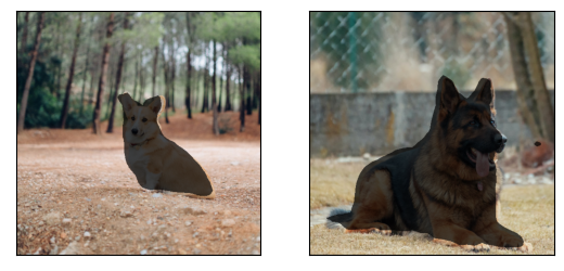
Here are some examples of visualizing the predictions of the LR-ASPP MobileNetV3-Large model:
We hope that you found this article interesting. We are looking forward to your feedback to see if this is the type of content you would like us to publish more often. If the community finds that such posts are useful, we will be happy to publish more articles that cover the implementation details of newly introduced Machine Learning models.