The National Football League (NFL) is America’s most popular sports league. Founded in 1920, the NFL developed the model for the successful modern sports league and is committed to advancing progress in the diagnosis, prevention, and treatment of sports-related injuries. Health and safety efforts include support for independent medical research and engineering advancements in addition to a commitment to better protect players and make the game safer. This includes enhancements to medical protocols and improvements to how our game is taught and played. For more information about the NFL’s health and safety efforts, see NFL Player Health and Safety.
We have partnered with AWS to develop the Digital Athlete program, where we use AWS machine learning (ML) services to identify potential risks coming from helmet-to-helmet, helmet-to-shoulder and other body parts, and helmet-to-ground collisions. As of this writing, there is no automated way to identify these collisions. An expert needs to review hours of game footage to visually identify impacts and compare that to the actual collisions reported during the game. Our team, in collaboration with AWS Professional Services and BioCore, is developing computer vision algorithms to analyze All-22 videos using Amazon SageMaker to help shape the future of American football and its players.
We planned to accomplish this objective in three steps: detect helmets, track detected helmets, and identify impacts to tracked helmets on the field. The tracking and impact detection workflows are beyond the scope of this post. This discussion focuses on helmet detection even under challenging conditions such as when players are obscured by other players for several frames and when video quality and video zoom effects change as the cameras track the action.
In this post, we discuss how state-of-the-art object detection model metrics don’t provide the full picture of where detection goes wrong, and how that motivated us to create a custom visualization for the entire play that shows the full story of helmet detection performance as a function of time within the play. This visualization has significantly improved our understanding of when and how our helmet detection algorithms fail.
Detection challenge
The challenges of a helmet detector model with respect to team play are three-fold:
- Helmet size is small compared to the image size in a typical clip of sideline or end zone view
- Precise detection is important to subsequently track the same helmet in future clips to correctly identify an impact, if any
- State-of-the-art object detection metrics collected from models don’t provide the full picture in the context of game plays
To address the first two challenges, we considered object detection algorithms that work well on relatively smaller objects and emphasize more on accuracy than speed.
To address the third challenge, we introduced a custom visualization technique that focused on some of the shortcomings of the conventional model metrics, specifically the following:
- A frame-wise error analysis that captures missed and false detections
- A visual summary of stacked true positives, false positives, and false negatives per frame over time to assess model performance for the entire play
Dataset and modeling
We recently announced a Kaggle competition (NFL 1st and Future – Impact Detection) for ML experts around the world to contribute towards NFL research addressing the need for a computer vision system to detect on-field helmet impacts as part of the Digital Athlete platform. In this post, we use static images from the competition data as an example to build a helmet detection model. We used Amazon SageMaker Ground Truth to create the computer vision dataset that is as accurate as possible to build a solid platform.
We used the Kaggle API to download the data within the SageMaker notebook instance. For instructions on creating a notebook instance, see Create a Notebook Instance. We used an ml.P3.2xlarge instance with one GPU and 50 GB EBS volume for better data manipulation and training. For more information about instance types, see Available Instance Types.
We started with some basic EDA to explore the static images and corresponding annotations. The labeled image dataset consists of 9,947 labeled images (with 4,958 sideline and 4,989 end zone) and a CSV file named image_labels.csv that contains the labeled bounding boxes for all images. The labeled file contains 193,736 helmets (114,986 sideline and 78,750 end zone) with 9,825 unique plays.
There are five different helmet labels, including Blurred, Sideline, Partial, and Difficult. The following table summarizes each label’s percentage of occurrence.
| Helmet label type | Percentage of occurrence |
| Helmet | 66.98% |
| Helmet-Blurred | 17.31% |
| Helmet-Sideline | 7.76% |
| Helmet-Partial | 4.55% |
| Helmet-Difficult | 3.39% |
We considered all Helmet types to be the same for simplicity and did an 80/20 split to train and test in the modeling phase.
Next, we used FasterRCNN with ResNet50 FPN as our helmet detection model and used a pretrained model based on COCO data within a PyTorch framework. For more information about object detection in TorchVision, see TorchVision Object Detection Finetuning Tutorial. The network seemed like an ideal choice because it detects objects of relatively smaller size and has performed very well in multiple standard object detection competitions. The goal was not to build an award-winning helmet detection model, but to identify errors in specific images within an entire play with a relatively high-performing model.
Model performance metrics
We trained the model using the default PyTorch Conda environment pytorch_p36 within a SageMaker notebook instance. The Average Precision (AP) @[IoU=0.50:0.95] for the test set at the end of 10 epochs was 0.498, and Average Recall @@[IoU=0.50:0.95] was 0.56 and deemed excellent as an object detector.
We took the saved model and evaluated frame by frame on an entire play (for example, 57583_000082_Endzone). We used annotation labels for the entire play to evaluate frame by frame. The following graph is a plot of precision vs. recall for all the frames with mAP of 93.12% using object detection metrics package.
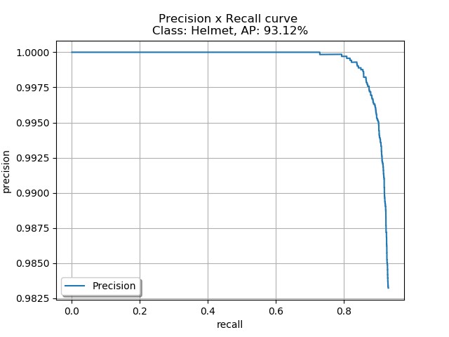
As evident from the plot, this is an excellent model and only fails if the helmet is either blurred or too difficult to detect even with expert eyes.
Next, we calculated the number of true positives, false positives, and false negatives for each frame of the 57583_000082_Endzone play. To match the predicted detection with ground truth annotations, we only considered predictions with scores higher than 0.9 and 0.25 IoU threshold between ground truth and the predicted bounding boxes. The conflicts between multiple detections for the same ground truth bounding boxes were resolved using a confidence score. Essentially, we only considered the highest confidence detections for multiple detections.
The number of ground truth helmets in each frame can vary between 18–22 for 57583_000082_Endzone, whereas our model predicted anywhere between 15–23 helmets. Therefore, even though our model is an excellent one, it did miss some helmets and made wrong predictions. Because false negatives or missed detections are more important for proper tracking of the players, we looked into the frames where we got too many false negatives.
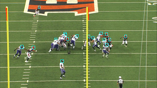
The following image shows an example where the model predicted every helmet correctly (depicted by the cyan boxes).
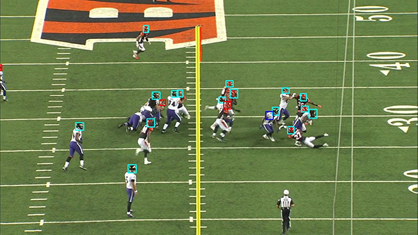
This next image shows where the model missed a few helmets (depicted by red boxes) and made wrong predictions (depicted by blue boxes).
To identify where and why a model is underperforming, it’s imperative to calculate the precision, recall, and F1-score for each frame and for the overall play. We got a precision of 0.97, recall of 0.93, and F1-score of 0.95 for the overall play, which definitely doesn’t provide the full picture of errors in a team play context. The following plot shows several false positives, false negatives on the right y-axis and precision, recall on the left y-axis against the individual frame number. It’s clear that our model did an excellent job overall except in the frames between approximately 100–300, where typically tackling happens in football plays. Unfortunately, most impacts or collisions happen in these frame ranges, and therefore we dug deeper into the error cases.
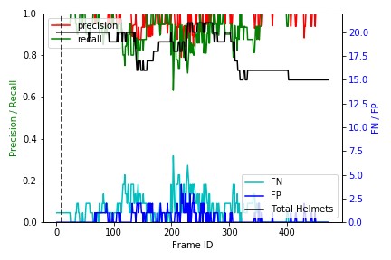
The following plot is a stacked bar representation of true positives (green area), false negatives (red area), and false positives (blue area) against individual frame numbers. The black bold line represents the total number of ground truth helmets in each frame. The dotted vertical black line represents the snap frame. An ideal helmet detector should detect each and every helmet in each frame, thereby covering the entire area with green. However, as you can see in the visualization, our model had limitations, which are clearly depicted both qualitatively and quantitatively in the visualization.
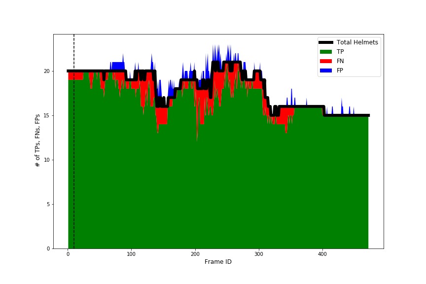
Therefore, this novel visualization gives us a tool to distinguish between an excellent helmet detector and a perfect helmet detector. It also provides a quick visual summary that allows us to compare the performance of the detector in different plays and quickly identify the temporal location and type of error the models are propagating. This can further be leveraged to assess improved helmet detector models after retraining.
To improve the helmet detector model, we could retrain the model using additional frames that are harder to detect into the training set, train for longer epochs, apply hyperparameter tuning, implement additional augmentation techniques, or incorporate other modeling strategies. At every step, we can use this stacked bar plot as a tool to assess the model quality in a team game perspective because it provides a visual summary that depicts where and how models are failing to perform against a perfect benchmark.
Prerequisites
To reproduce this analysis in your own environment, you must complete the following prerequisites:
It’s recommended to use an instance with GPU support, for example ml.p3.2xlarge. The EBS volume size should be around 50 GB in order to store all necessary data.
- Download the data from Kaggle using the Kaggle API.
Refer to the API credentials to retrieve and save the kaggle.json file on SageMaker within /home/ec2-user/.kaggle. For security reasons, make sure to change modes for accidental other users. See the following code:
pip install kaggle
mkdir /home/ec2-user/.kaggle
mv kaggle.json /home/ec2-user/.kaggle
chmod 600 ~/.kaggle/kaggle.json
kaggle competitions download -c nfl-impact-detection
Building the helmet detection model
The following code snippet shows the custom dataset class for helmets:
class DatasetHelmet(Dataset):

    def __init__(self, marking, image_ids, transforms=None, test=False):
        super().__init__()
        self.image_ids = image_ids
        self.marking = marking
        self.transforms = transforms
        self.test = test

    def __getitem__(self, index: int):
        image_id = self.image_ids[index]
        image, boxes, labels = self.load_image_and_boxes(index)
        num_boxes = len(boxes)
        if num_boxes > 0:
            target = {}
            new_boxes = torch.as_tensor(boxes, dtype=torch.float32)
            # there is only one class
            labels = torch.ones((num_boxes,), dtype=torch.int64)
            area = (new_boxes[:, 3] - new_boxes[:, 1]) * (new_boxes[:, 2] - new_boxes[:, 0])
            # suppose all instances are not crowd
            iscrowd = torch.zeros((num_boxes,), dtype=torch.int64)

            target['boxes'] = new_boxes
            target['labels'] = labels
            target['image_id'] = torch.tensor([index])
            target["area"] = area
            target["iscrowd"] = iscrowd
        else:
            target = {}

        if self.transforms is not None:
            image, target = self.transforms(image, target)
        return image, target

    def __len__(self) -> int:
        return self.image_ids.shape[0]

    def load_image_and_boxes(self, index):
        image_id = self.image_ids[index]
        TRAIN_ROOT_PATH = args.train + "images"
        image = cv2.imread(f'{TRAIN_ROOT_PATH}/{image_id}', cv2.IMREAD_COLOR).copy().astype(np.float32)
        image = cv2.cvtColor(image, cv2.COLOR_BGR2RGB).astype(np.float32)
        image /= 255.0
        records = self.marking[self.marking['image'] == image_id]
        boxes = records[['left', 'top', 'width', 'height']].values
        boxes[:, 2] = boxes[:, 0] + boxes[:, 2]
        boxes[:, 3] = boxes[:, 1] + boxes[:, 3]
        labels = records['label'].values
        return image, boxes, labels
The following code shows the main training function:
def main(args):
#     Read images label csv file
image_labels = pd.read_csv('/home/ec2-user/SageMaker/helmet_detection/input/image_labels.csv'
    # #     Split annotations into train and validation
    np.random.seed(0)
    image_names = np.random.permutation(image_labels.image.unique())
    valid_image_len = int(len(image_names)*0.2)
    images_valid = image_names[:valid_image_len]
    images_train = image_names[valid_image_len:]
    logging.info(f"images_valid {images_valid}, n images_train {images_train}")
    # Define train and validation datasets and data loaders
    TRAIN_ROOT_PATH = args.train

    train_dataset = DatasetHelmet(
        image_ids=images_train,
        marking=image_labels,
        transforms=get_transform(train=True),
        test=False,
    )
    validation_dataset = DatasetHelmet(
        image_ids=images_valid,
        marking=image_labels,
        transforms=get_transform(train=False),
        test=True,
    )
   data_loader = torch.utils.data.DataLoader(
        train_dataset, batch_size=args.batch_size, shuffle=True, num_workers=1,
        collate_fn=utils_torchvision.collate_fn
    )
    data_loader_valid = torch.utils.data.DataLoader(
        validation_dataset, batch_size=args.batch_size, shuffle=False, num_workers=1,
        collate_fn=utils_torchvision.collate_fn
    )
    print(f"We have {len(train_dataset)} images for training and {len(validation_dataset)} for validation")

    # Set up model
    device = torch.device('cuda') if torch.cuda.is_available() else torch.device('cpu')
    ## Our dataset has two classes only - helmet and not helmet
    num_classes = 2
    ## Get the model using our helper function
    model = get_model(num_classes)
    print(f"Loaded model")

    # Set up training
    start_epoch = 0
    end_epoch = args.epochs
    params = [p for p in model.parameters() if p.requires_grad]
    optimizer = torch.optim.SGD(params, lr=0.005,
                                momentum=0.9, weight_decay=0.0005)
    lr_scheduler = torch.optim.lr_scheduler.StepLR(optimizer,
                                                   step_size=3,
                                                   gamma=0.1)
    print(f"Loaded model parameters")

    ## if retraining from a checkpoint file
    if args.retrain:

        checkpoint = torch.load(os.path.join(args.model_dir, "model_checkpoint.pt"))
        model.load_state_dict(checkpoint['model_state_dict'])
        optimizer.load_state_dict(checkpoint['optimizer_state_dict'])
        start_epoch = checkpoint['epoch'] + 1
        end_epoch = start_epoch + args.epochs
        print('nLoaded checkpoint from epoch %d.n' % start_epoch)

    print(start_epoch, end_epoch)

    # Train model
    loss_epoch = []

    for epoch in range(start_epoch, end_epoch):
        # train for one epoch, printing every 1 iterations
        print(f"Training epoch {epoch}")
        train_one_epoch(model, optimizer, data_loader, data_loader_valid, device, epoch, loss_epoch, print_freq=1)

        # update the learning rate
        lr_scheduler.step()

        # evaluate on the test dataset
        evaluate(model, data_loader_valid, device=device, print_freq=1)
        # save checkpoint model after each epoch
        torch.save({
            'epoch': epoch,
            'model_state_dict': model.state_dict(),
            'optimizer_state_dict': optimizer.state_dict()
            }, os.path.join(args.model_dir, "model_checkpoint.pt"))


    # Save final model
    torch.save(model.state_dict(), os.path.join(args.model_dir, "model_helmet_frcnn.pt"))
    loss_df = pd.DataFrame(loss_epoch, columns=["train_loss", "val_loss"])
    loss_df.reset_index(inplace=True)
    loss_df = loss_df.rename(columns = {'index':'Epoch'})
    print(loss_df)
    loss_df.to_csv (os.path.join(args.model_dir, "loss_epoch.csv"), index = False, header=True)
Evaluating helmet detection model
Use the saved model to run predictions on an entire play. The following code is an example function to run evaluations:
def run_detection_eval_video(video_in, gtfile_name, model_path, full_video=True, subset_video=60, conf_thres=0.9, iou_threshold = 0.5):
    """ Run detection on video

    Args:
        video_in: Input video path
        gtfile_name: Ground Truth annotation json file name
        model_path: Location of the pretrained model.pt
        full_video: Bool to indicate whether to run the whole video, default = False
        subset_video: Number of frames to run detection on
        conf_thres = Only consider detections with score higher than conf_thres, default = 0.9
        iou_threshold = Match detection with ground trurh if iou is higher than iou_threshold, default = 0.5
    Returns:
        Predicted detection for all the frames in a video, evaluation for detection, a dataframe with bounding boxes for false negatives and false positives
        df_predictions (pandas.DataFrame): prediction of detected object for all frames
          with columns ['frame_id', 'class_id', 'score', 'x1', 'y1', 'x2', 'y2']
        eval_results (pandas.DataFrame): Count of total number of objects in gt and det, and tp, fn, fp for all frames
          with columns ['frame_id', 'num_object_gt', 'num_object_det', 'tp', 'fn', 'fp']
        fns (pandas.DataFrame): False negative records in a Pandas Dataframe for all frames
          with columns ['frame_id','class_id','x1','y1','x2','y2'],
          return empty if no false negatives
        fps (pandas.DataFrame): False positive records in a Pandas Dataframe for all frames
          with columns ['frame_id','class_id', 'score', 'x1','y1','x2','y2'],
          return empty if no false positives

    """
    # Capture the input video
    vid = cv2.VideoCapture(video_in)

    # Get video title
    vid_title = os.path.splitext(os.path.basename(video_in))[0]

    # Get total number of frames
    num_frames = vid.get(cv2.CAP_PROP_FRAME_COUNT)

    # load model
    num_classes = 2
    model = ObjectDetector.load_custom_model(model_path=model_path, num_classes=num_classes)
    print("Pretrained model loaded")

    # Get GT annotations
    gt_labels = pd.read_csv('/home/ec2-user/SageMaker/helmet_detection/input/train_labels.csv')
    video = os.path.basename(video_in)
    print("Processing video: ",video)
    labels = gt_labels[gt_labels['video']==video]

    # if running for the whole video, then change the size of subset_video with total number of frames
    if full_video:
        subset_video = int(num_frames)

    df_predictions = [] # predictions for whole video
    eval_results = [] # detection evaluations for the whole video
    fns = [] # false negative detections for the whole video
    fps = [] # false positive detections for the whole video

    for i in range(subset_video):

        ret, frame = vid.read()
        print("Processing frame#: {} running detection and evaluation for videos".format(i+1))

        # Get detection for this frame
        list_frame = [frame]
        dataset_frame = FramesDataset(list_frame)
        prediction = ObjectDetector.run_detection(dataset_frame, model)
        df_prediction = ObjectDetector.to_dataframe_highconf(prediction, conf_thres, i)
        df_predictions.append(df_prediction)

        # Get label for this frame
        cur_label = labels[labels['frame']==i+1] # get this frame's record
        cur_boxes = cur_label[['left','width','top','height']].values
        gt = ObjectDetector.get_gt_frame(i+1, cur_boxes)

        # Evaluate detection for this frame
        eval_result, fn, fp = ObjectDetector.evaluate_detections_iou(gt, df_prediction, iou_threshold)
        eval_results.append(eval_result)
        if fn is not None:
            fns.append(fn)
        if fp is not None:
            fps.append(fp)

    # Concatenate predictions, evaluation resutls, fns and fps for all frames of the video
    df_predictions = pd.concat(df_predictions)
    eval_results = pd.concat(eval_results)

    # Concatenate fns if not empty, otherwise create an empty dataframe
    if not fns:
        fns = pd.DataFrame()
    else:
        fns = pd.concat(fns)

    # Concatenate fps if not empty, otherwise create an empty dataframe
    if not fps:
        fps = pd.DataFrame()
    else:
        fps = pd.concat(fps)

    return df_predictions, eval_results, fns, fps
After we have evaluation results saved in a Pandas DataFrame, we can use the following code snippet to plot the stacked bar figure we described earlier:
pal = ["g","r","b"]
plt.figure(figsize=(12,8))
plt.stackplot(eval_det['frame_id'], eval_det['tp'], eval_det['fn'], eval_det['fp'],
              labels=['TP','FN','FP'], colors=pal)
plt.plot(eval_det['frame_id'], eval_det['num_object_gt'], color='k', linewidth=6, label='Total Helmets')
plt.legend(loc='best', fontsize=12)
plt.xlabel('Frame ID', fontsize=12)
plt.ylabel(' # of TPs, FNs, FPs', fontsize=12)
plt.axvline(x=snap_time, color='k', linestyle='--')
plt.savefig('/home/ec2-user/SageMaker/helmet_detection/output/stacked.png')
Conclusion
In this post, we showed how we used Amazon SageMaker to build a helmet detector model, ran error analysis on a team play context, and improved the detector model with better precision in the frames where it matters the most. With the visualization tool that we created, we could qualitatively and quantitatively assess the model accuracy in the entire play context. Furthermore, we could introduce additional training images and improve the model accuracy as depicted by both traditional state-of-the-art object detector metrics and our custom visualization.
With a near-perfect helmet detector model, our team is ready for the next step, which is tracking the players on the ground and detecting impacts using computer vision techniques. This will be discussed in a future post.
Readers are welcome to check out the Kaggle competition website and should be able to reproduce the results presented here with the code included in the post.
About the Authors
 Sam Huddleston is a Sr. Data Scientist at Biocore LLC, who serves as the Technology Lead for the NFL’s Digital Athlete program. Biocore is a team of world-class engineers based in Charlottesville, Virginia, that provides research, testing, biomechanics expertise, modeling and other engineering services to clients dedicated to the understanding and reduction of injury.
 Jayeeta Ghosh is a Data Scientist who works on AI/ML projects for AWS customers and helps solve customer business problems across industries using deep learning and cloud expertise.