With roads in developed countries like the US changing up to 15% annually, Mapillary addresses a growing demand for keeping maps updated by combining images from any camera into a 3D visualization of the world. Mapillary’s independent and collaborative approach enables anyone to collect, share, and use street-level images for improving maps, developing cities, and advancing the automotive industry.
Today, people and organizations all over the world have contributed more than 600 million images toward Mapillary’s mission of helping people understand the world’s places through images and making this data available, with clients and partners including the World Bank, HERE, and Toyota Research Institute.
Mapillary’s computer vision technology brings intelligence to maps in an unprecedented way, increasing our overall understanding of the world. Mapillary runs state-of-the-art semantic image analysis and image-based 3d modeling at scale and on all its images. In this post we discuss two recent works from Mapillary Research and their implementations in PyTorch – Seamless Scene Segmentation [1] and In-Place Activated BatchNorm [2] – generating Panoptic segmentation results and saving up to 50% of GPU memory during training, respectively.
Seamless Scene Segmentation
Github project page: https://github.com/mapillary/seamseg/
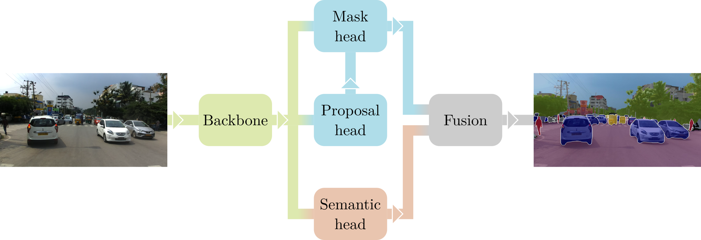
The objective of Seamless Scene Segmentation is to predict a “panoptic” segmentation [3] from an image, that is a complete labeling where each pixel is assigned with a class id and, where possible, an instance id. Like many modern CNNs dealing with instance detection and segmentation, we adopt the Mask R-CNN framework [4], using ResNet50 + FPN [5] as a backbone. This architecture works in two stages: first, the “Proposal Head” selects a set of candidate bounding boxes on the image (i.e. the proposals) that could contain an object; then, the “Mask Head” focuses on each proposal, predicting its class and segmentation mask. The output of this process is a “sparse” instance segmentation, covering only the parts of the image that contain countable objects (e.g. cars and pedestrians).
To complete our panoptic approach coined Seamless Scene Segmentation, we add a third stage to Mask R-CNN. Stemming from the same backbone, the “Semantic Head” predicts a dense semantic segmentation over the whole image, also accounting for the uncountable or amorphous classes (e.g. road and sky). The outputs of the Mask and Semantic heads are finally fused using a simple non-maximum suppression algorithm to generate the final panoptic prediction. All details about the actual network architecture, used losses and underlying math can be found at the project website for our CVPR 2019 paper [1].
While several versions of Mask R-CNN are publicly available, including an official implementation written in Caffe2, at Mapillary we decided to build Seamless Scene Segmentation from scratch using PyTorch, in order to have full control and understanding of the whole pipeline. While doing so we encountered a couple of main stumbling blocks, and had to come up with some creative workarounds we are going to describe next.
Dealing with variable-sized tensors
Something that sets aside panoptic segmentation networks from traditional CNNs is the prevalence of variable-sized data. In fact, many of the quantities we are dealing with cannot be easily represented with fixed sized tensors: each image contains a different number of objects, the Proposal head can produce a different number of proposals for each image, and the images themselves can have different sizes. While this is not a problem per-se – one could just process images one at a time – we would still like to exploit batch-level parallelism as much as possible. Furthermore, when performing distributed training with multiple GPUs, DistributedDataParallel expects its inputs to be batched, uniformly-sized tensors.
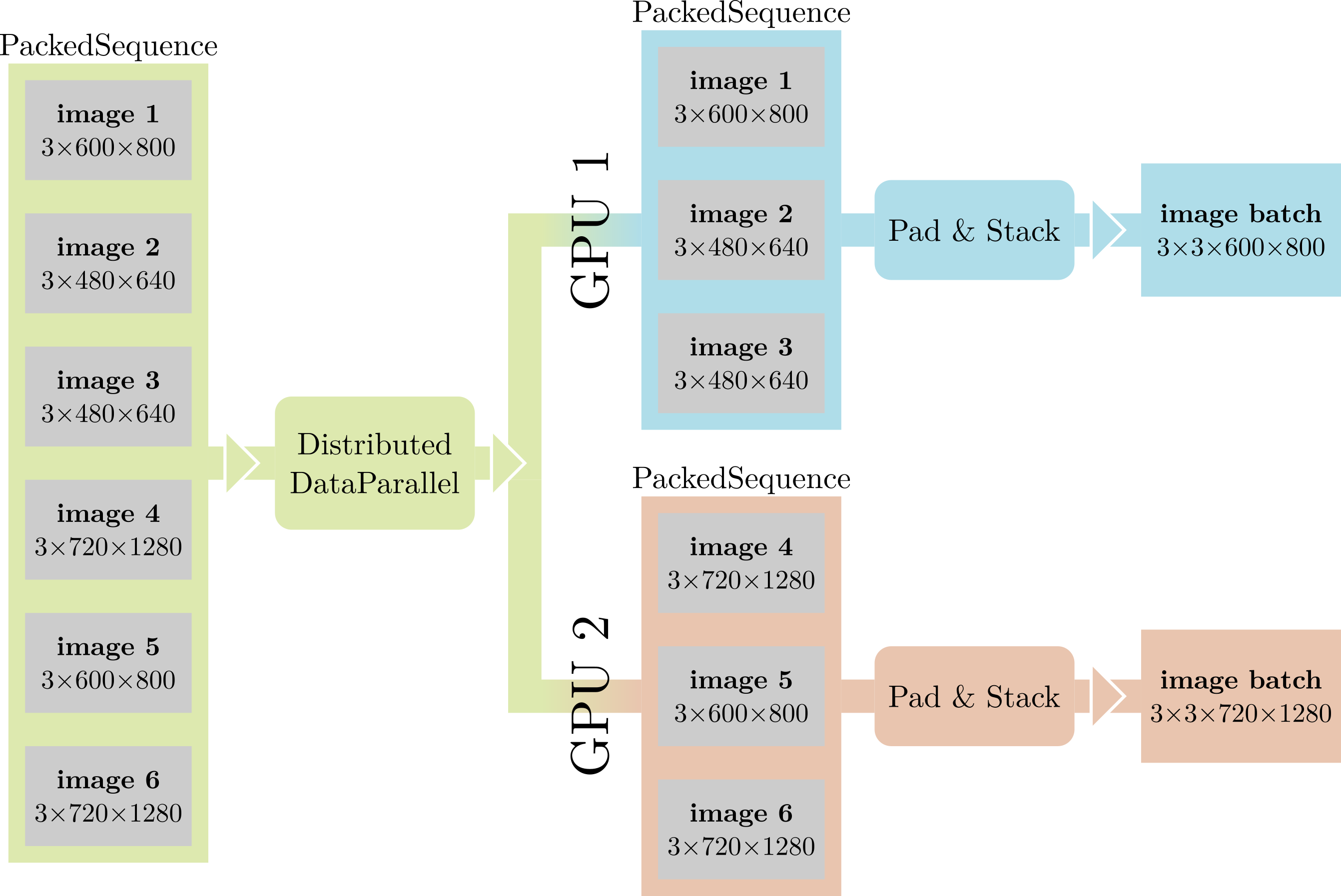
Our solution to these issues is to wrap each batch of variable-sized tensors in a PackedSequence. PackedSequence is little more than a glorified list class for tensors, tagging its contents as “related”, ensuring that they all share the same type, and providing useful methods like moving all the tensors to a particular device, etc. When performing light-weight operations that wouldn’t be much faster with batch-level parallelism, we simply iterate over the contents of the PackedSequence in a for loop. When performance is crucial, e.g. in the body of the network, we simply concatenate the contents of the PackedSequence, adding zero padding as required (like in RNNs with variable-length inputs), and keeping track of the original dimensions of each tensor.
PackedSequences also help us deal with the second problem highlighted above. We slightly modify DistributedDataParallel to recognize PackedSequence inputs, splitting them in equally sized chunks and distributing their contents across the GPUs.
Asymmetric computational graphs with Distributed Data Parallel
Another, perhaps more subtle, peculiarity of our network is that it can generate asymmetric computational graphs across GPUs. In fact, some of the modules that compose the network are “optional”, in the sense that they are not always computed for all images. As an example, when the Proposal head doesn’t output any proposal, the Mask head is not traversed at all. If we are training on multiple GPUs with DistributedDataParallel, this results in one of the replicas not computing gradients for the Mask head parameters.
Prior to PyTorch 1.1, this resulted in a crash, so we had to develop a workaround. Our simple but effective solution was to compute a “fake forward pass” when no actual forward is required, i.e. something like this:
def fake_forward():
    fake_input = get_correctly_shaped_fake_input()
    fake_output = mask_head(fake_input)
    fake_loss = fake_output.sum() * 0
    return fake_loss
Here, we generate a batch of bogus data, pass it through the Mask head, and return a loss that always back-progates zeros to all parameters.
Starting from PyTorch 1.1 this workaround is no longer required: by setting find_unused_parameters=True in the constructor, DistributedDataParallel is told to identify parameters whose gradients have not been computed by all replicas and correctly handle them. This leads to some substantial simplifications in our code base!
In-place Activated BatchNorm
Github project page: https://github.com/mapillary/inplace_abn/
Most researchers would probably agree that there are always constraints in terms of available GPU resources, regardless if their research lab has access to only a few or multiple thousands of GPUs. In a time where at Mapillary we still worked at rather few and mostly 12GB Titan X – style prosumer GPUs, we were searching for a solution that virtually enhances the usable memory during training, so we would be able to obtain and push state-of-the-art results on dense labeling tasks like semantic segmentation. In-place activated BatchNorm is enabling us to use up to 50% more memory (at little computational overhead) and is therefore deeply integrated in all our current projects (including Seamless Scene Segmentation described above).
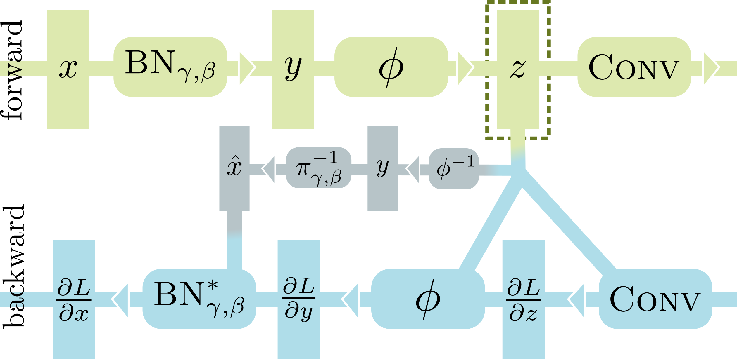
When processing a BN-Activation-Convolution sequence in the forward pass, most deep learning frameworks (including PyTorch) need to store two big buffers, i.e. the input x of BN and the input z of Conv. This is necessary because the standard implementations of the backward passes of BN and Conv depend on their inputs to calculate the gradients. Using InPlace-ABN to replace the BN-Activation sequence, we can safely discard x, thus saving up to 50% GPU memory at training time. To achieve this, we rewrite the backward pass of BN in terms of its output y, which is in turn reconstructed from z by inverting the activation function.
The only limitation of InPlace-ABN is that it requires using an invertible activation function, such as leaky relu or elu. Except for this, it can be used as a direct, drop-in replacement for BN+activation modules in any network. Our native CUDA implementation offers minimal computational overhead compared to PyTorch’s standard BN, and is available for anyone to use from here: https://github.com/mapillary/inplace_abn/.
Synchronized BN with asymmetric graphs and unbalanced batches
When training networks with synchronized SGD over multiple GPUs and/or multiple nodes, it’s common practice to compute BatchNorm statistics separately on each device. However, in our experience working with semantic and panoptic segmentation networks, we found that accumulating mean and variance across all workers can bring a substantial boost in accuracy. This is particularly true when dealing with small batches, like in Seamless Scene Segmentation where we train with a single, super-high resolution image per GPU.
InPlace-ABN supports synchronized operation over multiple GPUs and multiple nodes, and, since version 1.1, this can also be achieved in the standard PyTorch library using SyncBatchNorm. Compared to SyncBatchNorm, however, we support some additional functionality which is particularly important for Seamless Scene Segmentation: unbalanced batches and asymmetric graphs.
As mentioned before, Mask R-CNN-like networks naturally give rise to variable-sized tensors. Thus, in InPlace-ABN we calculate synchronized statistics using a variant of the parallel algorithm described here, which properly takes into account the fact that each GPU can hold a different number of samples. PyTorch’s SyncBatchNorm is currently being revised to support this, and the improved functionality will be available in a future release.
Asymmetric graphs (in the sense mentioned above) are another complicating factor one has to deal with when creating a synchronized BatchNorm implementation. Luckily, PyTorch’s distributed group functionality allows us to restrict distributed communication to a subset of workers, easily excluding those that are currently inactive. The only missing piece is that, in order to create a distributed group, each process needs to know the ids of all processes that will participate in the group, and even processes that are not part of the group need to call the new_group() function. In InPlace-ABN we handle it with a function like this:
import torch
import torch.distributed as distributed

def active_group(active):
    """Initialize a distributed group where each process can independently decide whether to participate or not"""
    world_size = distributed.get_world_size()
    rank = distributed.get_rank()

    # Gather active status from all workers
    active = torch.tensor(rank if active else -1, dtype=torch.long, device=torch.cuda.current_device())
    active_workers = torch.empty(world_size, dtype=torch.long, device=torch.cuda.current_device())
    distributed.all_gather(list(active_workers.unbind(0)), active)

    # Create group
    active_workers = [int(i) for i in active_workers.tolist() if i != -1]
    group = distributed.new_group(active_workers)
    return group
First each process, including inactive ones, communicates its status to all others through an all_gather call, then it creates the distributed group with the shared information. In the actual implementation we also include a caching mechanism for groups, since new_group() is usually too expensive to call at each batch.