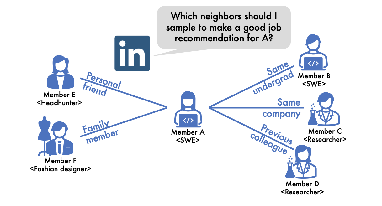
Figure 1: On LinkedIn, people are commonly connected with members from the same field who are likely to share skills and/or job preferences. Graph Convolutional Networks (GCNs) leverage this feature of the LinkedIn network and make better job recommendations by aggregating information from a member’s connections. For instance, to recommend a job to Member A, GCNs will aggregate information from Members B, C, and D who worked/are working in the same companies or have the same major.
TL;DR: Graph Convolutional Networks (GCNs) complement each node embedding with their neighboring node embeddings under a ‘homophily’ assumption, “connected nodes are relevant.” This leads to two critical problems when applying GCNs to real-world graphs: 1) scalability: numbers of neighboring nodes are sometimes too large to aggregate everything (e.g., Cristiano Ronaldo has 358 million connected accounts — his followers — on the Instagram’s member-to-member network), 2) low accuracy: nodes are sometimes connected with irrelevant nodes (e.g., people make connections with their personal friends who work in the totally different fields on LinkedIn). Here, we introduce a performance-adaptive sampling strategy for GCNs to solve both scalability and accuracy problems at once.
Graphs are ubiquitous. Any entities and interactions among them could be presented as graphs — nodes correspond to the individual entities and edges are generated between nodes when the corresponding entities have interactions between them. For instance, there are who-follows-whom graphs in social networks, who-pays-whom transaction networks in banking systems, and who-buys-which-products graphs in online malls. In addition to those originally graph-structured data, recently, few other computer science fields build new types of graphs by abstracting their concept (e.g., scene graphs in computer vision or knowledge graphs in NLP).
What are Graph Convolutional Networks?
As graphs contain rich contextual information — relationships among entities, various approaches have been proposed to include graph information in deep learning models. One of the most successful deep learning models combining graph information is Graph Convolutional Networks (GCNs) [1]. Intuitively, GCNs complement each node embeddings with their neighboring node embeddings, assuming neighboring nodes are relevant (we call this ‘homophily’), thus their information would help to improve a target node’s embedding. In Figure 1, on LinkedIn’s member-to-member networks, we refer to Member A‘s previous/current colleagues to make a job recommendation for Member A, assuming their jobs or skills are related to Member A‘s. GCNs aggregate neighboring node embeddings by borrowing the convolutional filter concept from Convolutional Neural Networks (CNNs) and replacing it with a first-order graph spectral filter.
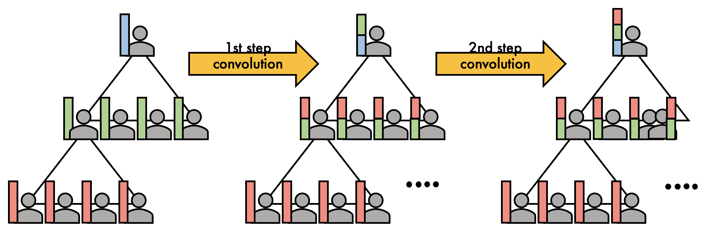
When (h_i^{(l)}) denotes the hidden embedding of node (v_i) in the (l)-th layer, one-step convolution (we also call it one-step aggregation or one-step message-passing) in GCNs is described as follows:
[h^{(l+1)}_i = alpha left( frac{1}{N(i)}sum_{j=1}^{N}a(v_i, v_j)h^{(l)}_jW^{(l)} right), quad l = 0,dots,L-1 tag{1}label{1}]where (a(v_i, v_j)) =1 when there is an edge from (v_i) to (v_j), otherwise 0; (N(i) = sum_{j=1}^{N} a(v_i, v_j)) is the degree of node (v_i); (alpha(cdot)) is a nonlinear function; (W^{(l)}) is the learnable transformation matrix. In short, GCNs average neighboring nodes (v_j)‘s embeddings (h_j^{(l)}), transform them with (W^{(l)}) and (alpha(cdot)), then update node (v_i)‘s embedding (h_i^{(l+1)}) using the aggregated and transformed neighboring embeddings. In practice, (h_i^{(0)}) is set with input node attributes and (h_i^{(L)}) is passed to an output layer specialized to a given downstream task. By stacking graph convolutional layers (L) times, (L)-layered GCNs complement each node embeddings with its neighboring nodes within (L) hops (Figure 2).
GCNs have garnered considerable attention as a powerful deep learning tool for representation learning of graph data. They demonstrate state-of-the-art performance on node classification, link prediction, and graph property prediction tasks. Currently, GCNs are one of most hot topics in graph mining and deep learning fields.
GCNs do not scale to large-scale real-world graphs.
However, when we adapt GCNs to million or billion-scaled real-world graphs (even trillion-scaled graphs for Google or Facebook), GCNs show a scalability issue. The main challenge comes from neighborhood expansion — GCNs expand neighbors recursively in the aggregation operations (i.e., convolution operations), leading to high computation and memory footprints. For instance, given a graph whose average degree is (d), (L)-layer GCNs access (d^L) neighbors per node on average (Figure 2). If the graph is dense or has many high degree nodes (e.g., Cristiano Ronaldo has 358 million followers on Instagram), GCNs need to aggregate a huge number of neighbors for most of the training/test examples.
The only way to alleviate this neighbor explosion problem is to sample a fixed number of neighbors in the aggregation operation, thereby regulating the computation time and memory usage. We first recast the original Equation (eqref{1}) as follows:
[h^{(l+1)}_i = alpha left( mathbb{E}_{jsim p(j|i)}[h^{(l)}_j]W^{(l)} right), quad l = 0,dots,L-1tag{2}label{2}]where (p(j|i) = frac{a(v_i, v_j)}{N(i)}) defines the probability of sampling (v_j) given (v_i). Then we approximate the expectation by Monte-Carlo sampling as follows [2]:
[h^{(l+1)}_i = alpha left( frac{1}{k}sum_{jsim p(j|i)}^{k}h^{(l)}_jW^{(l)} right), quad l = 0,dots,L-1tag{3}label{3}]where (k) is the number of sampled neighbors for each node. Now, we can regulate the GCNS’ computation costs using the sampling number (k).
GCN performance is affected by how neighbors are sampled, more specifically, how sampling policies — (q(j|i)), a probability of sampling a neighboring node (v_j) given a source node (v_i) — are defined. Various sampling policies [2-5] have been proposed to improve the GCN performance. Most of them target to minimize the variance caused by sampling (i.e., variance of the estimator (h^{(l+1)}_i) in Equation (eqref{3})). Variance minimization makes the aggregation of the sampled neighborhood to approximate the original aggregation of the full neighborhood. In other words, their sampling policies set the full neighborhood as the optimum they should approximate. But, is the full neighborhood the optimum?
Are all neighbors really helpful?
To answer this question, let’s go back to the motivation of the convolution operation in GCNs. When two nodes are connected with each other in graphs, we regard them as related to each other. Based on this ‘homophily’ assumption, GCNs aggregate neighboring nodes’ embeddings via the convolution operation to complement a target node’s embedding. So the convolution operation in GCNs will shine only when neighbors are informative for the task.
However, real-world graphs always contain unintended noisy neighbors. For example, in LinkedIn’s member-to-member networks, members might make connections not only with her colleagues working in the same field, but also with her family members or personal friends who may have totally different career paths (Figure 3). These family members or personal friends are uninformative for the job recommendation task. When their embeddings are aggregated into the target member’s embedding via the convolution operations, the recommendation quality becomes degraded. Thus, to fully enjoy benefits of the convolution operations, we need to filter out noisy neighbors.
How could we filter out noisy neighbors? We find the answer in the sampling policy: we sample neighbors only informative for a given task. How could we sample informative neighbors for the task? We train a sampler to maximize the target task’s performance (instead of minimizing sampling variance).
PASS: performance-adaptive sampling strategy for GCNs
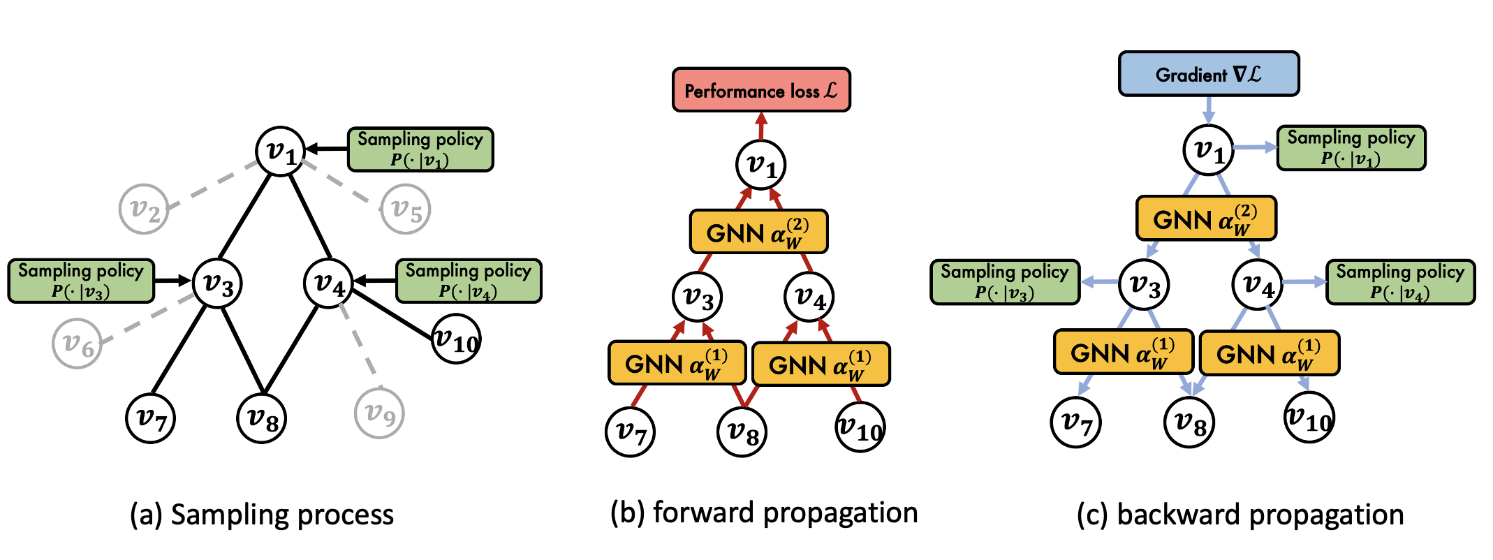
We propose PASS, a performance-adaptive sampling strategy that optimizes a sampling policy directly for GCN performance. The key idea behind our approach is that we learn a sampling policy by propagating gradients of the GCN performance loss through the non-differentiable sampling operation. We first describe a learnable sampling policy function and how it operates in the GCN. Then we describe how to learn the parameters of the sampling policy by back-propagating gradients through the sampling operation.
Sampling policy: Figure 4 shows an overview of PASS. In the forward pass, PASS samples neighbors with its sampling policy (Figure 4(a)), then propagates their embeddings through the GCN (Figure 4(b)). Here, we introduce our parameterized sampling policy (q^{(l)}(j|i)) that estimates the probability of sampling node (v_j) given node (v_i) at the (l)-th layer. The policy (q^{(l)}(j|i)) is composed of two methodologies, importance (q^{(l)}_{imp}(j|i)) and random sampling (q^{(l)}_{rand}(j|i)) as follows:
[q^{(l)}_{imp}(j|i) = (W_scdot h^{(l)}_i)cdot(W_scdot h^{(l)}_j)\q^{(l)}_{rand}(j|i) = frac{1}{N(i)}\
tilde{q}^{(l)}(j|i) = a_scdot[q^{(l)}_{imp}(j|i), quad q^{(l)}_{rand}(j|i)] \
q^{(l)}(j|i) = tilde{q}^{(l)}(j|i) / sum_{k=1}^{N(i)}tilde{q}^{(l)}(k|i)]
where (W_s) is a transformation matrix; (h^{(l)}_i) is the hidden embedding of node (v_i) at the (l)-th layer; (N(i)) is the degree of node (v_i); (a_s) is an attention vector; and (q^{(l)}(cdot|i)) is normalized to sum to 1. (W_s) and (a_s) are learnable parameters of our sampling policy, which will be updated toward performance improvement.
When a graph is well-clustered (i.e., less noisy neighbors), nodes are connected with all informative neighbors. Then random sampling becomes effective since its randomness helps aggregate diverse informative neighbors, thus preventing the GCN from overfitting. By capitalizing on both importance and random samplings, our sampling policy better generalizes across various graphs. Since we don’t know whether a given graph is well-clustered or not in advance, (a_s) learns which sampling methodology is more effective on a given task.
Training the Sampling Policy: after a forward pass with sampling, the GCN computes the performance loss (e.g., cross-entropy for node classification) then back-propagates gradients of the loss (Figure 4(c)). To learn a sampling policy maximizing the GCN performance, PASS trains the sampling policy based on gradients of the performance loss passed through the GCN. When (theta) denotes parameters ((W_s, a_s)) in our sampling policy (q^{(l)}_{theta}), we can write the sampling operation with (q^{(l)}_theta(j|i)) as follows:
[h^{(l+1)}_i = alpha_{W^{(l)}}(mathbb{E}_{jsim q^{(l)}_{theta}(j|i)}[h^{(l)}_j]), quad l = 0,dots,L-1]Before being fed as input to the GCN transformation (alpha_{W^{(l)}})((cdot)), the hidden embeddings (h^{(l)}_j) go through an expectation operation (mathbb{E}_{jsim q^{(l)}_{theta}(j|i)})[(cdot)] under the sampling policy, which is non-differentiable. To pass gradients of the loss through the expectation, we apply the log derivative trick [6], widely used in reinforcement learning to compute gradients of stochastic policies. Then the gradient (nabla_theta mathcal{L}) of the loss (mathcal{L}) w.r.t. the sampling policy (q^{(l)}_{theta(j|i)}) is computed as follows:
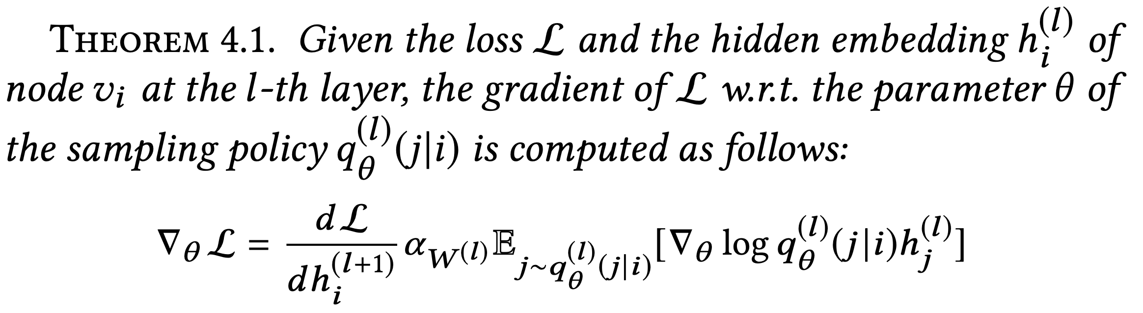
Based on Theorem 4.1, we pass the gradients of the GCN performance loss to the sampling policy through the non-differentiable sampling operation and optimize the sampling policy for the GCN performance. You can find proof of the theorem in our original paper. PASS optimizes the sampling policy jointly with the GCN parameters to minimize the task performance loss, resulting in a considerable performance improvement.
Experimental Results
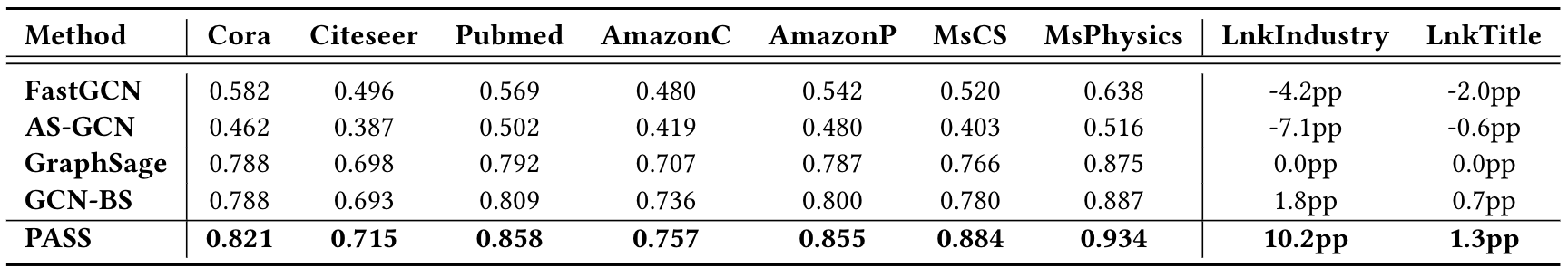
To examine the effectiveness of PASS, we run PASS on seven public benchmarks and two LinkedIn production datasets in comparison to four state-of-the-art sampling algorithms. GraphSage [2] samples neighbors randomly, while FastGCN [3], AS-GCN [4], and GCN-BS [5] do importance sampling with various sampling policy designs. Note that FastGCN, AS-GCN, and GCN-BS all target to minimize variance caused by neighborhood sampling. In Table 1, our proposed PASS method shows the highest accuracy among all baselines across all datasets on the node classification tasks. One interesting result is that GraphSage, which samples neighbors randomly, still shows good performance as compared to carefully designed importance sampling algorithms. The seven public datasets are well-clustered, which means most neighbors are relevant rather than noisy to a target node; thus there is not much room for improvement using importance sampling.
In the following experiment, we add noise to graphs. We investigate two different noise scenarios: 1) fake connections among existing nodes, and 2) fake neighbors with random feature vectors. These two scenarios are common in real-world graphs. The first “fake connection” scenario simulates connections made by mistake or unfit for the purpose (e.g., connections between family members in LinkedIn). The second “fake neighbor” scenario simulates fake accounts with random attributes used for fraudulent activities. For each node, we generate five true neighbors and five fake neighbors.
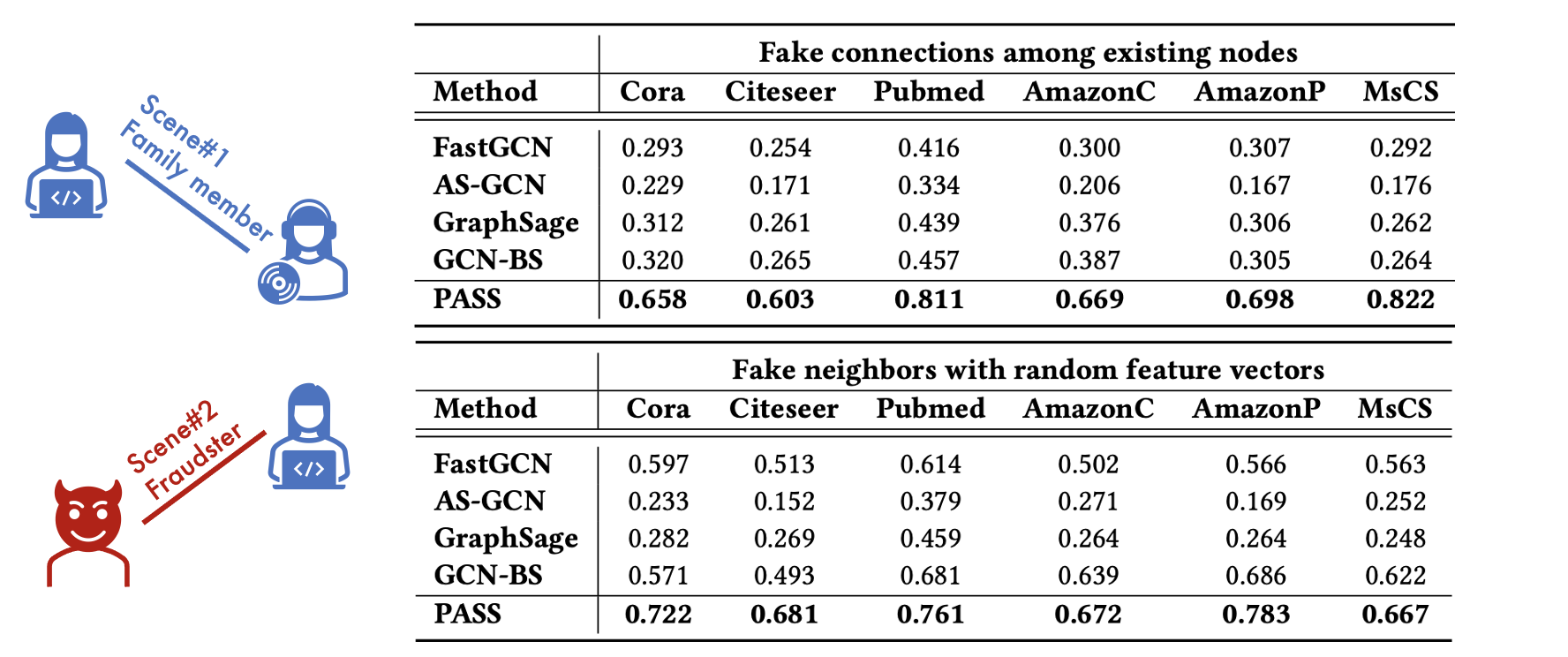
Table 2 shows that PASS consistently maintains high accuracy across all scenarios, while the performance of all other methods plummets. GraphSage, which gives the same sampling probability to true neighbors and fake neighbors, shows a sharp drop in accuracy. Other importance sampling-based methods, FastGCN, AS-GCN, and GCN-BS, also see a sharp drop in accuracy. They target to minimize sampling variance; thus they are likely to sample high-degree or dense-feature nodes, which help stabilize the variance, regardless of their relationship with the target node. Then, they all fail to distinguish fake neighbors from true neighbors. On the other hand, PASS learns which neighbors are informative or fake from gradients of the performance loss. These results show that the optimization of the sampling policy towards performance brings robustness to graph noise.
How does PASS learn which neighbors to sample?
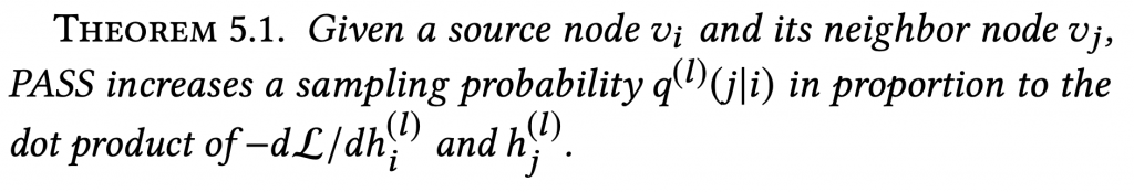
PASS demonstrates superior performance in sampling informative neighbors for a given task. How could PASS learn whether a neighbor is informative for the task? How could PASS decide a certain sampling probability for each neighbor? To understand how PASS actually works, we dissect the back-propagation process of PASS. In Theorem 5.1., we find out that, during the back-propagation phase, PASS measures the alignment between (-dmathcal{L}/dh^{(l)}_i) and (h^{(l)}_j) and increases the sampling probability (q^{(l)}(j|i)) in proportion to this alignment. Proof of Theorem 5.1. can be found in the original paper.
This is an intuitively reasonable learning mechanism. GCNs train their parameters to move the node embeddings (h^{(l)}_i) in the direction that minimizes the performance loss (mathcal{L}), i.e., the gradient (-dmathcal{L} / dh^{(l)}_i). PASS promotes this process by sampling neighbors whose embeddings are aligned with the gradient (-dmathcal{L}/dh^{(l)}_i). When (h^{(l)}_i) is aggregated with the embedding (h^{(l)}_j) of a sampled neighbor aligned with the gradient, it moves in the direction that reduces the loss (mathcal{L}).
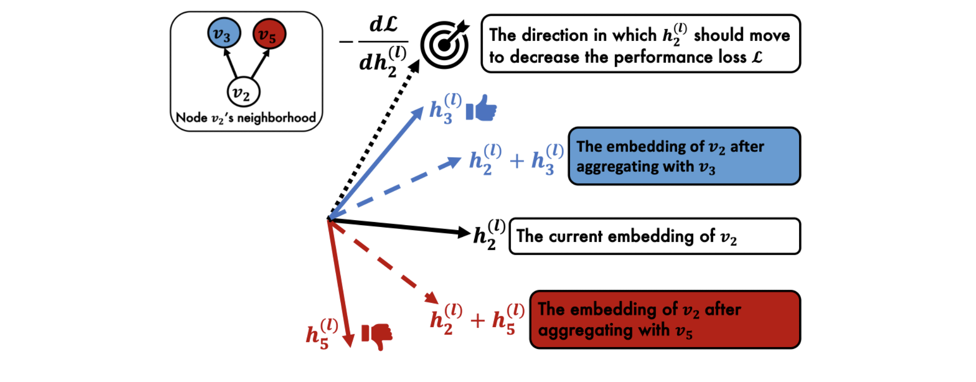
Let’s think about a simple example. In Figure 5, (h^{(l)}_3) is better aligned with (-dmathcal{L}/dh^{(l)}_2) than (h^{(l)}_5). Then PASS considers (v_3) more informative than (v_5) for (v_2) because node (v_3)’s embedding (h^{(l)}_3) helps (v_2)’s embedding (h^{(l)}_2) move in the direction (-dmathcal{L} / dh^{(l)}_2) that decreases the performance loss (mathcal{L}), while aggregating with node (v_5)’s embedding would move (h^{(l)}_2) in the opposite direction.
This reasoning process leads to two important considerations. First, it crystallizes our understanding of the aggregation operation in GCNs. The aggregation operation enables a node’s embedding to move towards its informative neighbors’ embeddings to reduce the performance loss. Second, this reasoning process shows the benefits of joint optimization of the GCN and sampling policy. Without optimizing the sampling policy jointly, the GCN depends solely on its parameters to move node embeddings towards the minimum performance loss. Joint optimization with the sampling policy helps the GCN to move the node embeddings more efficiently by aggregating with informative neighbors’ embeddings, leading to the minimum loss more efficiently.
PASS catches two birds, “accuracy” and “scalability”, with one stone.
Today, we introduced a novel sampling algorithm PASS for graph convolutional networks. By sampling neighbors informative for task performance, PASS improves both the accuracy and scalability of CGNs. In nine different real-world graphs, PASS consistently outperforms state-of-the-art samplers, being up to 10.4% more accurate. In the presence of graph noises, PASS shows up to 53.1% higher accuracy than the baselines, proving its ability to read the context and distinguish the noises. By dissecting the back-propagation process, PASS explains why a neighbor is considered informative and assigned a high sampling probability.
In this era of big data, new graphs and tasks are generated every day. Graphs become bigger and bigger, and different tasks require different relational information within the graphs. By sampling informative neighbors adaptively for a given task, PASS allows GCNs to be applied on larger-scale graphs and a more diverse range of tasks. We believe that PASS can bring even more impact on a wider range of users across academia and industry in the future.
Links: paper, video, slide, code will be released at the end of 2021.
If you would like to reference this article in an academic publication, please use this BibTeX:
@inproceedings{yoon2021performance,
  title={Performance-Adaptive Sampling Strategy Towards Fast and Accurate Graph Neural Networks},
  author={Yoon, Minji and Gervet, Th{'e}ophile and Shi, Baoxu and Niu, Sufeng and He, Qi and Yang, Jaewon},
  booktitle={Proceedings of the 27th ACM SIGKDD Conference on Knowledge Discovery & Data Mining},
  pages={2046--2056},
  year={2021}
}
References
- Thomas N Kipf and Max Welling. 2016. Semi-supervised classification with graph convolutional networks. arXiv preprint arXiv:1609.02907 (2016).
- Will Hamilton, Zhitao Ying, and Jure Leskovec. 2017. Inductive representation learning on large graphs. In Advances in neural information processing systems.
- Jie Chen, Tengfei Ma, and Cao Xiao. 2018. Fastgcn: fast learning with graph convolutional networks via importance sampling. arXiv preprint arXiv:1801.10247 (2018).
- Wenbing Huang, Tong Zhang, Yu Rong, and Junzhou Huang. 2018. Adaptive sampling towards fast graph representation learning. In Advances in neural information processing systems. 4558–4567
- Ziqi Liu, Zhengwei Wu, Zhiqiang Zhang, Jun Zhou, Shuang Yang, Le Song, and Yuan Qi. 2020. Bandit Samplers for Training Graph Neural Networks. arXiv preprint arXiv:2006.05806 (2020).
- Ronald J Williams. 1992. Simple statistical gradient-following algorithms for connectionist reinforcement learning. Machine learning 8, 3-4 (1992), 229–256.