Preventing customer churn by optimizing incentive programs using stochastic programming

In recent years, businesses are increasingly looking for ways to integrate the power of machine learning (ML) into business decision-making. This post demonstrates the use case of creating an optimal incentive program to offer customers identified as being at risk of leaving for a competitor, or churning. It extends a popular ML use case, predicting customer churn, and shows how to optimize an incentive program to address the real business goal of preventing customer churn. We use a large phone company for our use case.

Although it’s usual to treat this as a binary classification problem, the real world is less binary: people become likely to churn for some time before they actually churn. Loss of brand loyalty occurs some time before someone actually buys from a competitor. There’s frequently a slow rise in dissatisfaction over time before someone is finally driven to act. Providing the right incentive at the right time can reset a customer’s satisfaction.

This post builds on the post Gain customer insights using Amazon Aurora machine learning. There we met a telco CEO and heard his concern about customer churn. In that post, we moved from predicting customer churn to intervening in time to prevent it. We built a solution that integrates Amazon Aurora machine learning with the Amazon SageMaker built-in XGBoost algorithm to predict which customers will churn. We then integrated Amazon Comprehend to identify the customer’s sentiment when they called customer service. Lastly, we created a naïve incentive to offer customers identified as being at risk at the time they called.

In this post, we focus on replacing this naïve incentive with an optimized incentive program. Rather than using an abstract cost function, we optimize using the actual economic value of each customer and a limited incentive budget. We use a mathematical optimization approach to calculate the optimal incentive to offer each customer, based on our estimate of the probability that they’ll churn, and the probability that they’ll accept our incentive to stay.

Solution overview

Our incentive program is intended to be used in a system such as that described in the post Gain customer insights using Amazon Aurora machine learning. For simplicity, we’ve built this post so that it can run separately.

We use a Jupyter notebook running on an Amazon SageMaker notebook instance. Amazon SageMaker is a fully-managed service that enables developers and data scientists to quickly and easily build, train, and deploy ML models at any scale. In the Jupyter notebook, we first build and host an XGBoost model, identical to the one in the prior post. Then we run the optimization based on a given marketing budget and review the expected results.

Setting up the solution infrastructure

To set up the environment necessary to run this example in your own AWS account, follow Steps 0 and 1 in the post Simulate quantum systems on Amazon SageMaker to set up an Amazon SageMaker instance.

Then, as in Step 2, open a terminal. Enter the following command to copy the notebook to your Amazon SageMaker notebook instance:

wget https://aws-ml-blog.s3.amazonaws.com/artifacts/prevent_churn_by_optimizing_incentives/preventing_customer_churn_by_optimizing_incentives.ipynb

Alternatively, you can review a pre-run version of the notebook.

Building the XGBoost model

The first sections of the notebook—Setup, Data Exploration, Train, and Host, are the same as the sample notebook Amazon SageMaker Examples – Customer Churn. The exception is that we capture a copy of the data for later use and add a column to calculate each customer’s total spend.

At the end of these sections, we have a running XGBoost model on an Amazon SageMaker endpoint. We can use it to predict which customers will churn.

Assessing and optimizing

In this section of the post and accompanying notebook, we focus on assessing the XGBoost model and creating our optimal incentive program.

We can assess model performance by looking at the prediction scores, as shown in the original customer churn prediction post, Amazon SageMaker Examples – Customer Churn.

So how do we calculate the minimum incentive that will give the desired result? Rather than providing a single program to all customers, can we save money and gain a better outcome by using variable incentives, customized to a customer’s churn probability and value? And if so, how?

We can do so by building on components we’ve already developed.

Assigning costs to our predictions

The costs of churn for the mobile operator depend on the specific actions that the business takes. One common approach is to assign costs, treating each customer’s prediction as binary: they churn or don’t, we predicted correctly or we didn’t. To demonstrate this approach, we must make some assumptions. We assign the true negatives the cost of $0. Our model essentially correctly identified a happy customer in this case, and we won’t offer them an incentive. An alternative is to assign the actual value of the customer’s spend to the true negatives, because this is the customer’s contribution to our overall revenue.

False negatives are the most problematic because they incorrectly predict that a churning customer will stay. We lose the customer and have to pay all the costs of acquiring a replacement customer, including foregone revenue, advertising costs, administrative costs, point of sale costs, and likely a phone hardware subsidy. Such costs typically run in the hundreds of dollars, so for this use case, we assume $500 to be the cost for each false negative. For a better estimate, our marketing department should be able to give us a value to use for the overhead, and we have the actual customer spend for each customer in our dataset.

Finally, we give an incentive to customers that our model identifies as churning. For this post, we assume a one-time retention incentive of $50. This is the cost we apply to both true positive and false positive outcomes. In the case of false positives (the customer is happy, but the model mistakenly predicted churn), we waste the concession. We probably could have spent those dollars more effectively, but it’s possible we increased the loyalty of an already loyal customer, so that’s not so bad. We revise this approach later in this post.

Mapping the customer churn threshold

In previous versions of this notebook, we’ve shown the effect of false negatives that are substantially more costly than false positives. Instead of optimizing for error based on the number of customers, we’ve used a cost function that looks like the following equation:

cost_of_replacing_customer * FN(C) + customer_value * TN(C) + incentive_offered * FP(C) + incentive_offered * TP(C)

FN(C) means that the false negative percentage is a function of the cutoff, C, and similar for TN, FP, and TP. We want to find the cutoff, C, where the result of the expression is smallest.

We start by using the same values for all customers, to give us a starting point for discussion with the business. With our estimates, this equation becomes the following:

$500 * FN(C) + $0 * TN(C) + $50 * FP(C) + $50 * TP(C)

A straightforward way to understand the impact of these numbers is to simply run a simulation over a large number of possible cutoffs. We test 100 possible values, and produce the following graph.

The following output summarizes our results:

Cost is minimized near a cutoff of: 0.21000000000000002 for a cost of: $ 25800 for these 1500 customers.
Incentive is paid to 246 customers, for a total outlay of $ 12300
Total customer spend of these customers is $ 16324.36

The preceding chart shows how picking a threshold too low results in costs skyrocketing as all customers are given a retention incentive. Meanwhile, setting the threshold too high (such as 0.7 or above) results in too many lost customers, which ultimately grows to be nearly as costly. In between, there is a large grey area, where perhaps some more nuanced incentives would create better outcomes.

The overall cost can be minimized at $25,750 by setting the cutoff to 0.13, which is substantially better than the $100,000 or more we would expect to lose by not taking any action.

We can also calculate the dollar outlay of the program and compare to the total spend of the customers. Here we can see that paying the incentive to all predicted churn customers costs $13,750, and that these customers spend $183,700. (Your numbers may vary, depending on the specific customers chosen for the sample.)

What happens if we instead have a smaller budget for our campaign? We choose a budget of 1% of total customer monthly spend. The following output shows our results:

Total budget is: $895.90
Per customer incentive is $0.60

We can see that our cost changes. But it’s pretty clear that an incentive of approximately $0.60 is unlikely to change many people’s minds.

Can we do better? We could offer a range of incentives to customers that meet different criteria. For example, it’s worth more to the business to prevent a high spend customer from churning than a low spend customer. We could also target the grey area of customers that have less loyalty and could be swayed by another company’s advertising. We explore this in the following section.

Preventing customer churn using mathematical optimization of incentive programs

In this section, we use a more sophisticated approach to developing our customer retention program. We want to tailor our incentives to target the customers most likely to reconsider a churn decision.

Intuitively, we know that we don’t need to offer an incentive to customers with a low churn probability. Also, above some threshold, we’ve already lost the customer’s heart and mind, even if they haven’t actually left yet. So the best target for our incentive is between those two thresholds—these are the customers we can convince to stay.

The problem under investigation is inherently stochastic in that each customer might churn or not, and might accept the incentive (offer) or not. Stochastic programming [1, 2] is an approach for modeling optimization problems that involve uncertainty. Whereas deterministic optimization problems are formulated with known parameters, real-world problems almost invariably include parameters that are unknown at the time a decision should be made. An example would be the construction of an investment portfolio to maximize return. An efficient portfolio would be defined as the portfolio that maximizes the expected return for a given amount of risk (such as standard deviation), or the portfolio that minimizes the risk subject to a given expected return [3].

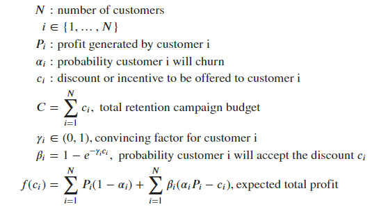
Our use case has the following elements:

• We know the number of customers, 𝑁.
• We can use the customer’s current spend as the (upper bound) estimate of the profit they generate, P.
• We can use the churn score from our ML model as an estimate of the probability of churn, alpha.
• We use 1% of our total revenue as our campaign budget, C.
• The probability that the customer is swayed, beta, depends on how convincing the incentive is to the customer, which we represent as 𝛾.
• The incentive, c, is what we want to calculate.

We set up our inputs: P (profit), alpha (our churn probabilities, from our preceding model), and C, our campaign budget. We then define the function we wish to optimize, f(c_i) being the expected total profit across the 𝑁 customers.

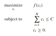
Our goal is to optimally allocate the discount 𝑐_𝑖 across the 𝑁 customers to maximize the expected total profit. Mathematically this is equivalent to the following optimization problem:

Now we can specify how likely we think each customer is to accept the offer and not churn—that is, how convincing they’ll find the incentive. We represent this as 𝛾 in the formulae.

Although this is a matter of business judgment, we can use the preceding graph to inform that judgment. In this case, the business believes that if the churn probability is below 0.55, they are unlikely to churn, even without an incentive; on the other hand, if the customer’s churn probability is above 0.95, the customer has little loyalty and is unlikely to be convinced. The real targets for the incentives are the customers with churn probability between 0.55–0.95.

We could include that business insight into the optimization by setting the value for the convincing factor 𝛾_𝑖 as follows:

• 𝛾_𝑖 = 100. This is equivalent to giving less importance as a deciding factor to the discount for customers whose churn probability is below 0.55 (they are loyal and less likely to churn), or greater than 0.95 (they will most likely leave despite the retention campaign).
• 𝛾_𝑖 = 1. This is equivalent to saying that the probability customer i will accept the discount is equal to 𝛽=1−𝑒^−C𝑖 for customers with churn probability between 0.55 and 0.95.

When we start to offer these incentives, we can log whether or not each customer accepts the offer and remains a customer. With that information, we can learn this function from experience, and use that learned function to develop the next set of incentives.

Solving the optimization problem

A variety of open-source solvers are available that can solve this optimization problem for us. Examples include SciPy scipy.optimize.minimize, or faster open-source solvers like GEKKO, which is what we use for this post. For large-scale problems, we would recommend using commercial optimization solvers like CPLEX or GUROBI.

After the optimization task has run, we check how much of our budget has been allocated.

The total spend is $1,000.00 compared to our budget of $1,000.00, and the total customer spend is $89,589.73 for 1,500 customers.

Now we evaluate the expected total profit for the following scenarios:

1. Optimal discount allocation, as calculated by our optimization algorithm
2. Uniform discount allocation: every customer is offered the same incentive
3. No discount

The following graph shows our outcomes.

Expected total profit compared to no campaign: 17%

Expected total profit compared to uniform discount allocation: 5%

Lastly, we add the discount to our customer data. We can see how the discount we offer varies across our customer base. The red vertical line shows the value of the uniform discount. The pattern of discounts we offer closely mirrors the pattern in the prediction scores, where many customers aren’t identified as likely churners, and a few are identified as highly likely to churn.

We can also see a sample of the discounts we’d be offering to individual customers. See the following table.

For each customer, we can see their total monthly spend and the optimal incentive to offer them. We can see that the discount varies by churn probability, and we’re assured that the incentive campaign fits within our budget.

Depending on the size of the total budget we allocate, we may occasionally find that we’re offering all customers a discount. This discount allocation problem reminds us of the water-filling algorithm in wireless communications [4,5], where the problem is of maximizing the mutual information between the input and the output of a channel composed of several subchannels (such as a frequency-selective channel, a time-varying channel, or a set of parallel subchannels arising from the use of multiple antennas at both sides of the link) with a global power constraint at the transmitter. More power is allocated to the channels with higher gains to maximize the sum of data rates or the capacity of all the channels. The solution to this class of problems can be interpreted as pouring a limited volume of water into a tank, the bottom of which has the stair levels determined by the inverse of the subchannel gains.

Unfortunately, our problem doesn’t have an intuitive explanation as for the water-filling problem. This is due to the fact that, because of the nature of the objective function, the system of equations and inequalities corresponding to the KKT conditions [6] doesn’t admit a closed form solution.

The optimal incentives calculated here are the result of an optimization routine designed to maximize an economic figure, which is the expected total profit. Although this approach provides a principled way for marketing teams to make systematic, quantitative, and analytics-driven decisions, it’s also important to recall that the objective function to be optimized is a proxy measure to the actual total profit. It goes without saying that we can’t compute the actual profit based on future decisions (this would paradoxically imply maximizing the actual return based on future values of the stocks). But we can explore new ideas using techniques such as the potential outcomes work [7], which we could use to design strategies for back-testing our solution.

Conclusion

We’ve now taken another step towards preventing customer churn. We built on a prior post in which we integrated our customer data with our ML model to predict churn. We can now experiment with variations on this optimization equation, and see the effect of different campaign budgets or even different theories of how they should be modeled.

To gather more data on effective incentives and customer behavior, we could also test several campaigns against different subsets of our customers. We can collect their responses—do they churn after being offered this incentive, or not—and use that data in a future ML model to further refine the incentives offered. We can use this data to learn what kinds of incentives convince customers with different characteristics to stay, and use that new function within this optimization.

We’ve empowered marketing teams with the tools to make data-driven decisions that they can quickly turn into action. This approach can drive fast iterations on incentive programs, moving at the speed with which our customers make decisions. Over to you, marketing!

Bibliography

About the Authors

Marco Guerriero, PhD, is a Practice Manager for Emergent Technologies and Intelligence Platform for AWS Professional Services. He loves working on ways for emergent technologies such as AI/ML, Big Data, IoT, Quantum, and more to help businesses across different industry verticals succeed within their innovation journey.

Veronika Megler, PhD, is Principal Data Scientist for Amazon.com Consumer Packaging. Until recently she, was the Principal Data Scientist for AWS Professional Services. She enjoys adapting innovative big data, AI, and ML technologies to help companies solve new problems, and to solve old problems more efficiently and effectively. Her work has lately been focused more heavily on economic impacts of ML models and exploring causality.

Oliver Boom is a London based consultant for the Emerging Technologies and Intelligent Platforms team at AWS. He enjoys solving large-scale analytics problems using big data, data science and dev ops, and loves working at the intersection of business and technology. In his spare time he enjoys language learning, music production and surfing.

Dr Sokratis Kartakis is a UK-based Data Science Consultant for AWS. He works with enterprise customers to help them adopt and productionize innovative Machine Learning (ML) solutions at scale solving challenging business problems. His focus areas are ML algorithms, ML Industrialization, and AI/MLOps. He enjoys spending time with his family outdoors and traveling to new destinations to discover new cultures.

Read More

Bibliography

[1] S. Uryasev, P. M. Pardalos, Stochastic Optimization: Algorithm and Applications, Kluwer Academic: Norwell, MA, USA, 2001. [2] John R. Birge and François V. Louveaux. Introduction to Stochastic Programming. Springer Verlag, New York, 1997. [3] Francis, J. C. and Kim, D. (2013). Modern portfolio theory: Foundations, analysis, and new developments (Vol. 795). John Wiley & Sons. [4] T. M. Cover and J. A. Thomas, Elements of Information Theory. New York: Wiley, 1991. [5] D. P. Palomar and J. R. Fonollosa, “Practical algorithms for a family of water-filling solutions,” IEEE Trans. Signal Process., vol. 53, no. 2, pp. 686–695, Feb. 2005. [6] S. Boyd and L. Vandenberghe. Convex optimization. Cambridge university press, 2004. [7] Imbens, G. W. and D. B. Rubin (2015): Causal Inference for Statistics, Social, and Biomedical Sciences, Cambridge University Press.About the Authors