Fig. 1: The safety envelope (in green) is an imaginary surface that separates the robot from all obstacles in its environment. As long as the robot never intersects the safety envelope, it is guaranteed to not collide with any obstacle. Our task is to estimate this envelope.
Safe navigation and obstacle detection
Consider the scene in Fig. 1 that a mobile robot wishes to navigate safely. The scene contains many obstacles such as walls, poles, and walking people. Obstacles could be arbitrarily distributed, their motion might be haphazard, and they may enter and leave the environment in an undetermined manner. This situation is commonly encountered in a variety of robotics tasks such as indoor and outdoor robot navigation, autonomous driving, and robot delivery. The robot must accurately and reliably detect all obstacles (static and dynamic) in the scene to avoid colliding with them and navigate safely. Therefore, it must estimate the safety envelope of the scene.
What is a safety envelope?
We define the safety envelope as an imaginary surface that separates the robot from all obstacles in its environment. As long as the robot never intersects the safety envelope, it is guaranteed to not collide with any obstacles! How can the robot accurately estimate the location of the safety envelope? Can it provide any guarantees about its ability to discover obstacles? In our recent paper published at RSS 2021, we answer these questions in the affirmative using a novel sensor called programmable light curtains.
What are light curtains?
A programmable light curtain is a 3D sensor recently invented at CMU. It can measure the depth of any user-specified 2D vertical surface (“curtain”) in the environment. A common strategy for 3D sensing is to use LiDARs. LiDARs have become ubiquitous in robotics and autonomous driving. However, they can be low resolution, expensive and slow. In contrast, light curtains are relatively inexpensive, faster, and of much higher resolution!
| LiDAR (Velodyne) | Light curtain |
|---|---|
| Low resolution (128 rows) | High resolution (1280 rows) |
| Expensive (~$100,000) | Inexpensive (~$1,000) |
| Slow (5-20 Hz) | Fast (60 Hz) |
| No control required | User control required |
Most importantly, light curtains are a controllable sensor: the user selects a vertical 2D surface, and the light curtain detects objects intersecting that surface. This is a fundamentally different sensing paradigm from LiDARs. LiDARs passively sense the entire scene without any user input. However, light curtains can be actively controlled by the user to focus their sensing capacity on specific regions of interest. While controllability is clearly a desirable feature, it also presents a unique challenge: light curtains require the user to select which locations to sense. How should we place light curtains to accurately estimate the safety envelope of a scene?
Random curtains can reliably discover obstacles
Suppose we have a scene with no prior knowledge of where the obstacles are. How should we place light curtains to discover them? Surprisingly, we answered this question by taking inspiration from heist films such as Ocean’s Twelve. In a scene from this movie shown in Fig. 3, the robber attempts to evade a museum’s security system consisting of randomly moving laser detectors. The robber needs to try extremely hard, literally bending over backward, to avoid intersecting the lasers. Although the robber managed to pull it off in the movie, it is clear that this would be virtually impossible in the real world.
Light curtains are nothing but moving laser detectors! Therefore, our insight is to place curtains at random locations in the scene. We refer to them as “random curtains”, as shown in Fig. 4. It turns out to be incredibly hard for (sufficiently large) obstacles to avoid getting detected by random curtains. We place random curtains to quickly discover unknown objects and estimate the safety envelope of the scene.
In the section on theoretical analysis of random curtains near the end of this blog post, we will present a novel analytical technique that actually computes the probability of random curtains intersecting and detecting obstacles. The analytical probabilities act as safety guarantees for our perception system towards detecting and avoiding obstacles.
Forecasting safety envelopes

Assume that we have already estimated the safety envelope in the current timestep. As objects move and the scene changes with time, we wish to estimate the safety envelope for the next timestep. In this case, it may be inefficient to explore the scene from scratch by randomly placing curtains. Instead, we use machine learning to train a neural network to forecast how the safety envelope will evolve in the next timestep. The inputs to the network are all light curtain measurements from previous timesteps. The output is the predicted change in the envelope’s position in the next timestep. We use DAgger [Ross et. al. 2011], a standard imitation learning algorithm, to train such a forecasting model from data. By predicting how the safety envelope will move, we can directly sense the locations where obstacles are anticipated to be and efficiently track the safety envelope.
Active light curtain placement pipeline

Our overall pipeline for placing light curtains to estimate and track the safety envelope is as follows. Given previous light curtain measurements, we train a neural network to forecast how the safety envelope of the scene will evolve in the next timestep. We then place light curtains to sense the predicted locations. At the same time, we place random light curtains to discover obstacles and update our predictions. Finally, the light curtain measurements are input back to the forecasting method, closing the loop.
Real-world results
Here is our method in action in the real world! The scene consists of multiple people walking in front of the light curtain device at various speeds and in different patterns. Our method, which combines learning-based forecasting and random curtain placement, tries to estimate the safety envelope of this dynamic scene at each timestep.
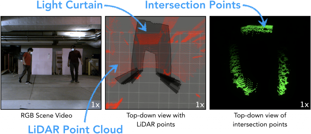
The middle video shows the light curtain placed at the estimated location of the safety envelope in black. It also shows a LiDAR point cloud in red, used only for visualization purposes (our method only uses light curtain measurements). The video on the right shows intersection points, i.e. the points detected by the light curtain when it intersects object surfaces in green. These are aggregated across multiple frames to visualize the motion of obstacles.
Brisk Walking

Relaxed Walking
Many people (structured walking)
Many people (haphazard, occluded walking)
Fast motion
In all of the above videos, the light curtain is able to accurately estimate the safety envelope and produce a large number of intersection points. Due to the guarantees of high detection probability, our method generalizes to a varying number of obstacles (one vs. two vs. five people), a large range of motion (relaxed vs. brisk vs. extremely fast and sudden motion), and different patterns of motion (structured vs. complicated and haphazard).
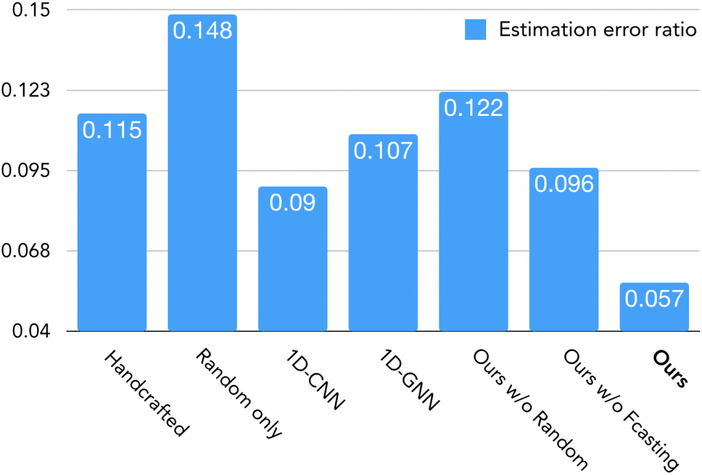
Fig. 7 shows a quantitative analysis of our method compared to various baselines. We compute the Huber loss (related to the “smooth-L1 loss“) of the ratio between the predicted and true safety envelope location. We compare against a non-learning based handcrafted baseline. The baseline carefully alternates between moving the light curtain forward and backward, resulting in “hugging” the obstacles. We also compare against using only random curtains and using various neural network architectures. We include ablation experiments that remove one component of our method at a time (random curtains and forecasting) to demonstrate that both are crucial to our performance. Our method outperforms all baselines. Please see our paper for more experiments and evaluation metrics.
Theoretical analysis of random curtain detection
Previously, we mentioned that random light curtains can detect obstacles with a high probability. Can we perform any theoretical analysis to actually compute this probability? Can we compute the probability of a random curtain detecting an obstacle of a given shape, size, and location? If so, these probabilities can act as safety guarantees that help certify the ability of our perception system to detect and avoid obstacles. Before we begin analyzing random curtains, we must first understand how they are generated.
Constraint Graph and generating random curtains
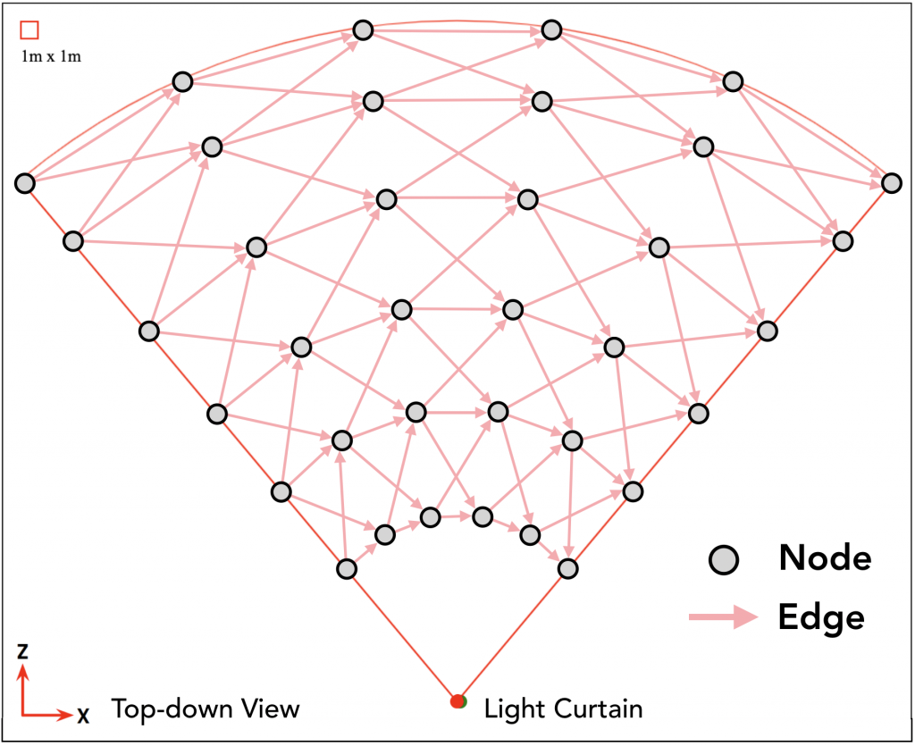
In order to generate any light curtain, we need to account for the physical constraints of the light curtain device. These are encoded into a constraint graph (see Fig. 8). The nodes of the graph represent locations where the light curtain might be placed. The nodes are organized into “camera rays” indexed by (t in {1, dots, T}) from left to right. A light curtain is created by imaging one node per ray, from left to right. An edge exists between two nodes if they can be imaged consecutively.
What decides whether an edge exists between two nodes? The light curtain device contains a rotating mirror that redirects and shoots light into the scene. By specifying the angle of rotation, light can be beamed at the desired locations to be imaged. However, the mirror, being a physical device, has velocity and acceleration limits. Therefore, we add an edge between two nodes only if the mirror can rotate fast enough to image those two locations one after the other.
This means that any path in the constraint graph connecting the leftmost ray (t=1) to the rightmost ray (t=T) represents a feasible light curtain! Furthermore, random curtains can be generated by performing a random walk through the graph. The random walk is performed by starting from a node on the leftmost ray. In each iteration, a node on the next ray is randomly sampled among the neighbors of the current node from some probability distribution (e.g. uniform distribution). This process is repeated till the rightmost ray is reached. Fig. 9 shows examples of actual random curtains generated this way.
Computing detection probability using Dynamic Programming
Assume that we are given the shape, size, and location of an obstacle (blue–red shape in Fig. 10). Some random curtains will intersect and detect the obstacle (detections are shown in yellow), but other random curtains will miss the obstacle. Can we compute the probability of detection?
A naive approach would be to enumerate the set of all feasible light curtains and sum the probabilities of sampling those curtains that detect the object. Unfortunately, this is impractical because the number of feasible curtains is exponentially large! Another approach is to use Monte Carlo sampling for estimating the detection probability. In this method, we sample a large number of random curtains and output the fraction of the sampled curtains that detect the obstacle. While this approach is simple, we will show later that it requires a large number of samples to be drawn, and only produces stochastic estimates of the true probability.
Instead, we have developed an analytical and efficient approach to compute the detection probability, using dynamic programming. We first divide the overall problem into multiple sub-problems. Let us represent (mathbf{x}_t) to be a node on the (t)-th ray. Let us define (P_mathrm{det}(mathbf{x}_t)) to be the the probability that “sub-curtains” i.e. partial random curtains starting from node (mathbf{x}_t) and ending at a rightmost node will detect the obstacle. We wish to compute (P_mathrm{det}(cdot)) for every node in the constraint graph. Conveniently, these sub-problems satisfy a recursive relationship! If the obstacle is detected at node (mathbf{x}_t), (P_mathrm{det}(mathbf{x}_t)) is trivially equal to (1). If not, it is equal to the sum of detection probabilities of sub-curtains starting at (mathbf{x}_t)’s child nodes (mathbf{x}_{t+1}), weighted by the probability (P(mathbf{x}_t rightarrow mathbf{x}_{t+1})) of transitioning to (mathbf{x}_{t+1}). This is expressed by the equation below.
$$
P_mathrm{det}(mathbf{x}_{t}) =
begin{cases}
1 & text{if obstacle is detected at node } mathbf{x}_{t}\
sum_{mathbf{x}_{t+1}} P(mathbf{x}_{t} rightarrow mathbf{x}_{t+1})~P_mathrm{det}(mathbf{x}_{t+1}) & text{otherwise}
end{cases} tag{1}
$$
In order to apply dynamic programming, we start at nodes on the rightmost ray (T). (P_mathrm{det}(cdot)) for these nodes is simply (1) or (0), depending on whether the obstacle is detected at these locations or not. Then, we iterate over all nodes in the graph from right to left (see Fig. 11) and apply the recursive formula in Eqn. 1. Once we have the sub-curtain detection probabilities for the leftmost nodes, the overall detection probability is simply (sum_{mathbf{x}_1} P_mathrm{init}(mathbf{x}_1)~P_mathrm{det}(mathbf{x}_1)), where (P_mathrm{init}(mathbf{x}_1)) is the probability of sampling (mathbf{x}_1) as the starting node of the random curtain.
Note that our method computes the true detection probability precisely — there is no stochasticity or noise in the estimates. It is also very efficient: we only need to iterate over all nodes and edges in the graph once.
An example of random curtain analysis
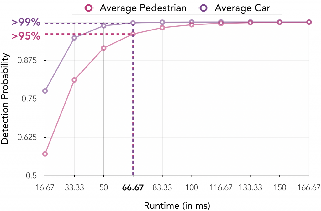
Let us look at an example of random curtain analysis in Fig. 12. The X-axis shows the time taken to place multiple random curtains at 60 Hz. The Y-axis shows the detection probability of an average-sized car and an average-sized pedestrian. Average sizes were computed from KITTI, a large-scale autonomous driving benchmark dataset. Let (p) be the probability of detecting an obstacle by a single random curtain. If (n) curtains are sampled independently and placed, the probability that at least one of them will detect the object is (1-(1-p)^n), which increases exponentially with (n). Thanks to the high speed of light curtains, within as low as 67 milliseconds, we are able to guarantee the detection of an average-sized pedestrian with more than 95% probability and an average-sized car with more than 99% probability!
Comparison to sampling-based estimation
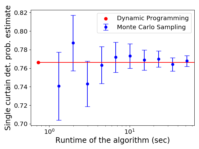
In traditional Monte Carlo estimation, we sample a large number of random curtains by performing multiple forward passes through the constraint graph. Then, we output the fraction of the sampled curtains that detect the obstacle. This produces an unbiased estimate of the detection probability, with a variance that decreases with the number of samples used. Fig. 13 show the estimates produced by each method with 95% confidence intervals, versus their runtime (in log-scale). Monte Carlo (MC) sampling produces noisy estimate of the true probability whereas our dynamic programming (DP) approach produces precise estimates (zero uncertainty); such precise estimates are useful for reliably evaluating the safety and robustness of our perception system. Furthermore, DP is orders of magnitude faster (takes 0.8 seconds) than MC since MC requires a large number of samples to converge to our estimate.
We have created an interactive web-based demo of random curtain analysis! The user can draw any shape, size, and location of the obstacle. The demo runs dynamic programming to compute the random curtain detection probability and displays the analysis. The demo also generates random curtains and visualizes detections of the obstacle. Click on the link to check it out!
Conclusion
We presented a method to estimate the safety envelope of a scene: a hypothetical surface that separates the robot from all obstacles in the environment. We used programmable light curtains, an actively controllable, resource-efficient sensor to directly estimate the safety envelope. Using a dynamic programming-based approach, we showed that random light curtains can discover obstacles with high-probability guarantees. We combined this with a machine learning-based forecasting method to efficiently track the safety envelope. This enables our robot perception system to accurately estimate safety envelopes, while our probabilistic guarantees help certify its accuracy and safety. This work is a step towards safe robot navigation using inexpensive controllable sensors.
Further reading
If you’re interested in more details, please check out the links to the full paper, the project website, talk, demo, and more!
Citation
This blog post is based on the following paper :
Siddharth Ancha, Gaurav Pathak, Srinivasa Narasimhan, and David Held.
Active Safety Envelopes using Light Curtains with Probabilistic Guarantees.
In Proceedings of Robotics: Science and Systems (RSS), July 2021.
Acknowledgements
Thanks to David Held, Srinivasa Narasimhan and Paul Liang for feedback on this post!
This material is based upon work supported by the National Science Foundation under Grants No. IIS-1849154, IIS-1900821 and by the United States Air Force and DARPA under Contract No. FA8750-18-C-0092. All opinions, findings, and conclusions or recommendations expressed in this post are those of the author(s) and do not necessarily reflect the views of Carnegie Mellon University, National Science Foundation, United States Air Force and DARPA.