Various machine learning (ML) optimizations are possible at every stage of the flow during or after training. Model compiling is one optimization that creates a more efficient implementation of a trained model. In 2018, we launched Amazon SageMaker Neo to compile machine learning models for many frameworks and many platforms. We created the ML compiler service so that you don’t need to set up compiler software, such as TVM, XLA, Glow, TensorRT, or OpenVINO, or be concerned with tuning the compiler for best model performance.
Since then, we have updated Neo to support more operators and expand model coverage for TensorFlow, PyTorch, and Apache MXNet (incubating). In October 2020, we made an internal change to allow a model to be partially compiled for CPU and GPU targets. Prior to this change, Neo could only compile a model if all the operators from the model could be compiled. With this change, Neo can figure out which part of the model can be compiled, and generates a model artifact combining the compiled and non-compiled parts. The combined model artifact can be used by SageMaker managed inference endpoints. The non-compiled parts of the model continue running in the framework, while the compiled parts run natively on CPU or GPU. As a result, many more models can see increased inference speeds in SageMaker when they are compiled with Neo.
The interface to model compiling has remained unchanged. This post shows the resulting model performance improvements and the mechanics behind how they work. For a step-by-step tutorial on using Neo to compile a model and deploy in SageMaker managed endpoints, see these notebook examples: Tensorflow mnist, PyTorch VGG19, and MxNet SSD Mobilenet.
Partially compiling a model
In the following example, I took a pre-trained alpha pose model alpha_pose_resnet101_v1b_coco from the GluonCV model zoo and compiled it with Neo. I saved the model from the model zoo into the following two files:
alpha_pose_resnet101_v1b_coco-0000.params
alpha_pose_resnet101_v1b_coco-symbol.json
Then I packed these files into a tar.gz file in an Amazon Simple Storage Service (Amazon S3) bucket and used Neo to compile the model.
Neo compiled the model and created a tar.gz file in an S3 bucket. After downloading and unpacking, I have two files that represent the compiled model (in addition to some other files, which I don’t discuss in detail):
compiled-0000.params
compiled-symbol.json
The compiled-symbol.json file contains all nodes of the model graph and edges between nodes. In this case, the Neo compiler service created five optimized subgraphs in the alpha pose model. Each subgraph is represented by the _tvm_subgraph_op node in the model graph. I can use a simple grep command to discover number of subgraphs:
$ cat compiled-symbol.json |grep _tvm_subgraph_op
      "op": "_tvm_subgraph_op",
      "op": "_tvm_subgraph_op",
      "op": "_tvm_subgraph_op",
      "op": "_tvm_subgraph_op",
      "op": "_tvm_subgraph_op",
Next I use a slightly more complex grep command to show you how many ops of each kind are in this model, which ops are in the subgraphs, and which ops are not. The following code block contains 11 instances of the Activation op in all the subgraphs (line is indented), four instances of the broadcast_like op not in any subgraph (line is not indented), and five instances of the subgraph_op:
$ cat compiled-symbol.json | grep ""op"" | grep -v null | sort | uniq -c

     11               "op": "Activation",
    106               "op": "BatchNorm",
    107               "op": "Convolution",
      8               "op": "FullyConnected",
      1               "op": "Pooling",
      9               "op": "Reshape",
      4               "op": "_contrib_AdaptiveAvgPooling2D",
     33               "op": "elemwise_add",
      4               "op": "elemwise_mul",
      8               "op": "expand_dims",
     99               "op": "relu",
      3               "op": "transpose",
      5       "op": "_tvm_subgraph_op",
      4       "op": "broadcast_like",
In a future update of Neo, we may add support to compile the broadcast_like op, in which case the model is entirely compiled.
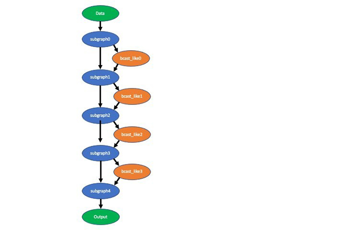
You can visualize the compiled model with the graph visualization tool. The following visualization depicts the partially compiled alpha pose model. This shows you the data flow between the subgraphs and ops not compiled (broadcast_like).
Even though I’m showing you an example of the Neo compiled artifacts from the GluonCV model zoo, the same subgraph concept applies to the TensorFlow and PyTorch compiled artifacts as well. The format of compiled artifacts is different in these other frameworks.
The following table shows the measured latency speedup of this partially compiled model compared with a non-compiled model on one CPU and one GPU Amazon Elastic Compute Cloud (Amazon EC2) instance. The speedup is specific to the model and instance type because the performance gain achieved varies with model architecture and platform.
| Instance | Speedup |
| c5.9xl | 1.28 |
| g4dn.xl | 1.23 |
Next I deployed the compiled model to SageMaker endpoints using the SageMaker inference container, which is integrated with TVM runtime.
Speedup numbers across common models and frameworks
The following table lists latency speedup that you might see from a few common models in all three frameworks in CPU and GPU instances.
| Framework | Model | Instance | Speedup |
| TensorFlow | resnet50 | c5.9xl | 2.86 |
| TensorFlow | resnet50 | g4dn.xl | 1.86 |
| PyTorch | inception v3 | c5.4xl | 3.03 |
| PyTorch | inception v3 | p3.2xl | 3.53 |
| MXNet | yolo3 | m5.12xl | 1.26 |
| MXNet | yolo3 | g4dn.xl | 1.11 |
These numbers are only general guidelines, as opposed to performance expectations for your specific model and instance choice. The numbers in the table are measured at the instance level and don’t include time spent on preprocessing and postprocessing. In SageMaker hosting, preprocessing and postprocessing can also take time, and is worth looking into in your overall optimization strategy.
How compiling works
In all frameworks (PyTorch, TensorFlow, and MXNet), we start by analyzing the model. We look at clusters of operators that are compilable, and fuse these into subgraphs. We avoid creating too many subgraphs using heuristics. Running subgraphs has an extra cost of data copy and launch overhead. If all operators are compilable in a model, the entire model is a single subgraph with all the operators.
In all frameworks, we use TVM to compile the subgraphs. On Nvidia GPU instance types (g4, p3, p2), we use the TensorRT integration feature of TVM to further identify operators in the subgraphs that can be compiled by TensorRT, creating subgraphs within a subgraph. A hybrid model running on these GPU instances may use the framework runtime, TVM runtime, and TensorRT runtime.
In some dynamic model cases, we use the relayVM from TVM, which has native support for dynamic tensor shape and control flow operators. This allows fully ahead-of-time compilation for models such as Mask R-CNN. As of this writing, compilers such as XLA or TensorRT use just-in-time to handle dynamic tensor shapes, which incur extra compiling cost whenever a new tensor shape is present when running a model.
At the subgraph level, TVM uses a framework-specific front-end component to convert the subgraph into relay IR (intermediate language). Relay IR is very expressive and can support data types, variables, control flow, function calls, and highly parallelizable compute operations such as matrix multiplication.
From relay IR, TVM does two types of optimizations: graph level and node or tensor level. One kind of graph-level optimization is to fuse two or more nodes together to avoid extra data copy. This is especially useful when GPU is involved because launching a small kernel too many times is very expensive. Another kind of graph-level optimization is to change the way a multi-dimensional array is stored in memory based on the operators involved. An example is that the conv2D operator used in computer vision models prefers the 4-D array sent to it to be in the NCHW format. Yet another optimization is to pre-compute parts of the subgraph at compile time (constant folding). By rewriting the graph in certain ways, TVM can improve the run speed of the model.
Node- or tensor-level optimization is about generating more efficient code for the operator. For example, the most optimal way of doing conv2D depends on the size of the 4-D array in each dimension. TVM can take advantage of this knowledge and generate code based on the hardware attributes of the target device, such as L1 cache size and CPU or GPU instruction scheduling policies.
Summary
Neo can now compile nearly all ML models from TensorFlow, PyTorch, and MXNet frameworks for SageMaker CPU and GPU instances. We continue to tune and optimize Neo. If you have any questions or comments, use the Amazon SageMaker Discussion Forums or send an email to amazon-neo-feedback@amazon.com.
About the Author
 Wei Xiao is a Principle Engineer working on the optimization of machine learning systems in the Amazon AWS AI org. Previously he worked on distributed systems and relational databases in Amazon and Microsoft for many years.