Posted by Frederick Liu and Garima Pruthi, Software Engineers, Google Research
The quality of a machine learning (ML) model’s training data can have a significant impact on its performance. One measure of data quality is the notion of influence, i.e., the degree to which a given training example affects the model and its predictive performance. And while influence is a well-known concept to ML researchers, the complexity behind deep learning models, coupled with their growing size, features and datasets, have made the quantification of influence difficult.
A few methods have been proposed recently to quantify influence. Some rely on changes in accuracy when retraining with one or several data points dropped, and some use established statistical methods, e.g., influence functions that estimate the impact of perturbing input points or representer methods that decompose a prediction into an importance weighted combination of training examples. Still other approaches require use of additional estimators, such as data valuation using reinforcement learning. Though these approaches are theoretically sound, their use in products has been limited by the resources needed to run them at scale or the additional burdens they place on training.
In “Estimating Training Data Influence by Tracing Gradient Descent”, published as a spotlight paper at NeurIPS 2020, we proposed TracIn, a simple scalable approach to tackle this challenge. The idea behind TracIn is straightforward — trace the training process to capture changes in prediction as individual training examples are visited. TracIn is effective in finding mislabeled examples and outliers from a variety of datasets, and is useful in explaining predictions in terms of training examples (as opposed to features) by assigning an influence score to each training example.
The Ideas Underlying TracIn
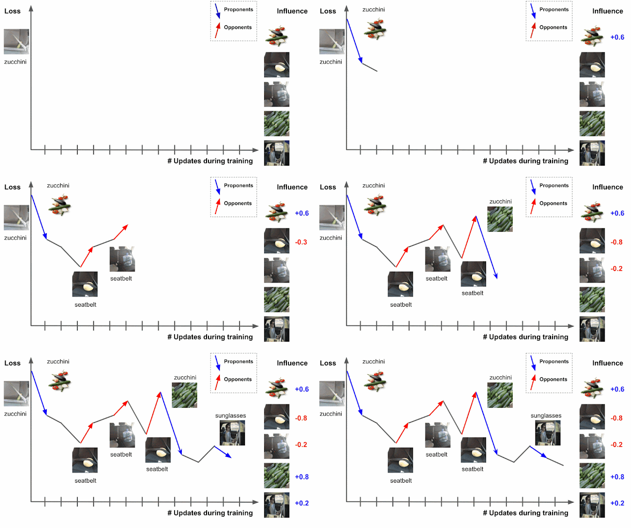
Deep learning algorithms are typically trained using an algorithm called stochastic gradient descent (SGD), or a variant of it. SGD operates by making multiple passes over the data and making modifications to the model parameters that locally reduce the loss (i.e., the model’s objective) with each pass. An example of this is demonstrated for an image classification task in the figure below, where the model’s task is to predict the subject of the test image on the left (“zucchini”). As the model progresses through training, it is exposed to various training examples that affect the loss on the test image, where the loss is a function both of the prediction score and the actual label — the higher the prediction score for zucchini, the lower the loss.
 |
| Estimating training data influence of the images on the right by tracing the loss change of the zucchini in the seatbelt image during training. |
Suppose that the test example is known at training time and that the training process visited each training example one at a time. During the training, visiting a specific training example would change the model’s parameters, and that change would then modify the prediction/loss on the test example. If one could trace the training example through the process, then the change in loss or prediction on the test example could be attributed to the training example in question, where the influence of a training example would be the cumulative attribution across visits to the training example.
There are two types of relevant training examples. Those that reduce loss, like the images of zucchinis above, are called proponents, while those that increase loss, like the images of seatbelts, are called opponents. In the example above, the image labeled “sunglasses” is also a proponent, because it has a seatbelt in the image, but is labeled as “sunglasses,” driving the model to better distinguish between zucchini and seatbelts.
In practice, the test example is unknown at training time, a limitation that can be overcome by using the checkpoints output by the learning algorithm as a sketch of the training process. Another challenge is that the learning algorithm typically visits several points at once, not individually, which requires a method to disentangle the relative contributions of each training example. This can be done by applying pointwise loss gradients. Together, these two strategies capture the TracIn method, which can be reduced to the simple form of the dot product of loss gradients of the test and training examples, weighted by the learning rate, and summed across checkpoints.
 |
| The simple expression for TracIn influence. The dot product of loss gradients of training example (z) and test example (z’) is weighted by learning rate (ηi) at different checkpoints and summed up. |
Alternatively, one could instead examine the influence on the prediction score, which would be useful if the test example has no label. This form simply requires the substitution of the loss gradient at the test example with the prediction gradient.
Computing Top Influence Examples
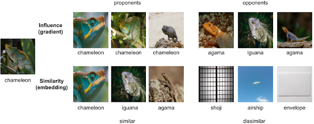
We illustrate the utility of TracIn by first calculating the loss gradient vector for some training data and a test example for a specific classification — an image of a chameleon — and then leveraging a standard k-nearest neighbors library to retrieve the top proponents and opponents. The top opponents indicate the chameleon’s ability to blend in! For comparison, we also show the k nearest neighbors with embeddings from the penultimate layer. Proponents are images that are not only similar, but also belong to the same class, and opponents are similar images but in a different class. Note that there isn’t an explicit enforcement on whether proponents or opponents belong to the same class.
 |
| Top row: Top proponents and opponents of influence vectors. Bottom row: Most similar and dissimilar examples of embedding vectors from the penultimate layer. |
Clustering
The simplistic breakdown of the loss of the test example into training example influences given by TracIn also suggests that the loss (or prediction) from any gradient descent based neural model can be expressed as a sum of similarities in the space of gradients. Recent work has demonstrated that this functional form is similar to that of a kernel, implying that this gradient similarity described here can be applied to other similarity tasks, like clustering.
In this case, TracIn can be used as a similarity function within a clustering algorithm. To bound the similarity metric so that it can be converted to a distance measure (1 – similarity), we normalize the gradient vectors to have unit norm. Below, we apply TracIn clustering on images of zucchini to obtain finer clusters.
Identifying Outliers with Self-Influence
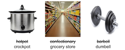
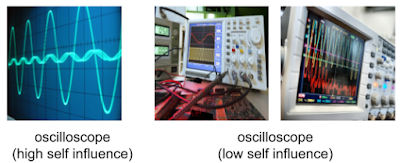
Finally, we can also use TracIn to identify outliers that exhibit a high self-influence, i.e., the influence of a training point on its own prediction. This happens either when the example is mislabeled or rare, both of which make it difficult for the model to generalize over the example. Below are some examples with high self-influence.
 |
| Mislabeled examples. Assigned labels are striked out, correct labels are at bottom. |
Applications
Having no requirement other than being trained using SGD (or related variants), TracIn is task-independent and applicable to a variety of models. For example, we have used TracIn to study training data for a deep learning model used to parse queries to the Google Assistant, queries of the kind “set my alarm for 7AM”. We were intrigued to see that the top opponent for the query “disable my alarm” with an alarm active on the device, was “disable my timer”, also with an alarm active on the device. This suggests that Assistant users often interchange the words “timer” and “alarm”. TracIn helped us interpret the Assistant data.
More examples can be found in the paper, including a regression task on structured data and a number of text classification tasks.
Conclusion
TracIn is a simple, easy-to-implement, scalable way to compute the influence of training data examples on individual predictions or to find rare and mislabeled training examples. For implementation references of the method, you can find a link to code examples for images from the github linked in the paper.
Acknowledgements
The NeurIPS paper was jointly co-authored with Satyen Kale and Mukund Sundararajan (corresponding author). A special thanks to Binbin Xiong for providing various conceptual and implementation insights. We also thank Qiqi Yan and Salem Haykal for numerous discussions. Images throughout this post sourced from Getty Images.


