We upgrade pixels into PIPs: “Persistent Independent Particles”. With this representation, we track any pixel over time, and overcome visibility issues with a learned temporal prior.
Motion estimation is a fundamental task of computer vision, with extremely broad applications. By tracking something, you can build models of its various properties: shape, texture, articulation, dynamics, affordances, and so on. More fine-grained tracking allows more fine-grained understanding. For robots, fine-grained tracking also enables fine-grained manipulation. Even setting aside downstream AI-related applications, motion tracks are directly useful for video editing applications — making realistic edits to a person or object in a video demands precise-as-possible tracking of the pixels, across an indefinite timespan.
There are a variety of methods for tracking objects (at the level of segmentation masks or bounding boxes), or for tracking certain points in certain categories (e.g., the joints of a person), but there are actually very few options for general-purpose fine-grained tracking. In this domain, the dominant approaches are feature matching and optical flow. The feature matching approach is: compute a feature for the target on the first frame, then compute features for pixels in other frames, and then compute “matches” using feature similarity (i.e., nearest neighbors). This often works well, but does not take into account temporal context, like smoothness of motion. The optical flow approach is: compute a dense “motion field” that relates each pair of frames, and then do some post-processing to link the fields together. Optical flow is very powerful, but since it only describes motion for a pair of frames at a time, it cannot produce useful outputs for targets that undergo multi-frame occlusion. “Occlusion” means our view is obstructed, and we need to guess the target’s location from context.
Around the year 2006, Peter Sand and Seth Teller proposed an alternative to flow-based and feature-based methods, called a “particle video.” This approach aims to represent a video with a set of particles that move across multiple frames. Their proposed method did not handle occlusions, but in our view, they laid the groundwork for treating pixels as persistent entities, with multi-frame trajectories and long-range temporal priors.
Inspired by their work, we propose Persistent Independent Particles (PIPs), a new particle video method. Our method takes a video as input, along with the ( (x, y) ) coordinate of a target to track, and produces the target’s trajectory as output. The model can be queried for any number of particles, at any positions.
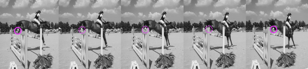
You may notice in our visualizations that the PIP trajectories often leave the video bounds. We treat pixels flying out-of-bounds as just another “occlusion.” This type of robustness is exactly what is missing from feature-based and flow-based methods.
Let’s step through how we achieved this.
How does it work?
At a high level, our method makes an extreme trade-off between spatial awareness and temporal awareness: we estimate the trajectory of every target independently. This extreme choice allows us to devote the majority of parameters into a module that simultaneously learns (1) temporal priors, and (2) an iterative inference mechanism that searches for the target pixel’s location in all input frames. Related work on optical flow estimation typically uses the opposite approach: they estimate the motion of all pixels simultaneously (using maximal spatial context), for just 2 frames at a time (using minimal temporal context).
Given the ( (x_1,y_1) ) coordinate of the target on the first frame, our concrete goal is to estimate the target’s full trajectory over (T) frames: ( (x_1,y_1), ldots, (x_T,y_T) ).
We start by initializing a zero-velocity estimate. This means copying the initial coordinate to every timestep.

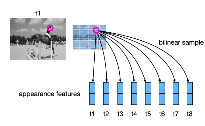
To track the target, we need to know what it looks like, so we compute appearance features for all the frames (using a CNN), and initialize the target’s appearance trajectory with a bilinear sample at the given coordinate on the first frame. (The “bilinear sample” step extracts a feature vector at a subpixel location in the spatial map of features.)
Our inference process will proceed by iteratively refining the sequence of positions, and sequence of appearance features, until they (hopefully) match the true trajectory of the target. This idea is illustrated in the video below: at initialization, only “timestep 1” has the correct location of the target (since this was given), and gradually, the model “locks on” to the target in all frames.
Our model’s job is to produce updates (i.e., deltas) for the positions and features, so that the trajectory tracks the target on every frame. A critical detail here is that we ask our model to produce these updates for multiple timesteps simultaneously. This allows us to “catch” a target after it re-emerges from an occluder, and “fill in” the missing part of the trajectory.
There are many ways to implement this, but for fast training and good generalization, we need to carefully select what information we provide to the model.
The main source of information we provide to the model is: measurements of local appearance similarity. We obtain these measurements using cross correlation (i.e., dot products), computed at multiple scales. When the target is visible, it should show up as a strong peak in at least one of the similarity maps. Also, when we are “locked on”, the peak should be in the middle of the map. This is illustrated in the animation below.
The second source of information we provide to the model is: the estimated trajectory itself. This allows the model to impose a temporal prior, and fix up parts of the trajectory where the local similarity information was ambiguous.
Finally, we allow the model to inspect the feature vector of the target, in case it might learn different strategies for different types of features. For example, depending on the scale or texture of the target, it may adjust the way it uses information from the multi-scale similarity maps.
For the model architecture, we elected to use an MLP-Mixer, which we found to have a good trade-off between model capacity, training time, and generalization. We also tried convolutional models and transformers, but the convolutional models could not fit the data as well as the MLP-Mixer, and the transformers took too long to train.
We trained the model in synthetic data that we made (based on an existing optical flow dataset), where we could provide multi-frame ground-truth for targets that undergo occlusions. The animation below shows the kind of data we trained on. You might say the data looks crazy — but that’s the point! If you can’t get real data, your best bet is synthetic data with extremely high diversity.
After training for a couple days on this data, the model starts to work on real videos.
Results
In the paper, we provide some quantitative analysis, showing that it works better than existing methods. It’s certainly not perfect — on keypoint tracking, the model works about 6/10 times, so there is a lot of room for improvement. The baselines are at around 5/10 or less.
The idea here is: pick a point on the first frame, and try to locate that same point in other frames of the video. This is a hard task especially when the point gets occluded.
Baseline methods tend to get stuck on occluders, since they do not use multi-frame temporal context. For example, here is the output of a state-of-the-art optical flow method, on the same video and same target.
We have had fun trying the model on various videos, and observing the estimated trajectories. Sometimes they are surprisingly complex, since the target’s actual motion is subtly entangled with camera motion.
Visualizing the trajectories more densely gives mesmerizing results. Notice that the model even tracks ripples and specularities in the water.
Despite the fact that each particle trajectory is estimated independently of the others, they show surprisingly accurate grouping. Notice that the background particles all move together.
What’s next?
Our method upgrades pixels into PIPs: “Persistent Independent Particles.” This independence assumption, however, is probably not what we want in general. In ongoing work, we are trying to incorporate context across particles, so that confident particles can help the unconfident ones, and so that we track at multiple levels of granularity simultaneously.
We have released our code and model weights on GitHub. We encourage you to try our demo.py! If you are interested in building on our method, the provided tests, visualizations, and training scripts should make that easy. Or, if you are working on a video-based method that currently relies on optical flow, you may want to try our PIP trajectories as a replacement, which should give a better signal under occlusions.
We hope that our work opens up long-range fine-grained tracking of “anything.” For more details, please check out our project page and paper.