Training Production AI Models with PyTorch 2.0

1. Introduction

PyTorch 2.0 (abbreviated as PT2) can significantly improve the training and inference performance of an AI model using a compiler called_ torch.compile_ while being 100% backward compatible with PyTorch 1.x. There have been reports on how PT2 improves the performance of common benchmarks (e.g., huggingface’s diffusers). In this blog, we discuss our experiences in applying PT2 to production _AI models _at Meta.

2. Background

2.1 Why is automatic performance optimization important for production?

Performance is particularly important for production—e.g, even a 5% reduction in the training time of a heavily used model can translate to substantial savings in GPU cost and data-center power. Another important metric is development efficiency, which measures how many engineer-months are required to bring a model to production. Typically, a significant part of this bring-up effort is spent on manual _performance tuning such as rewriting GPU kernels to improve the training speed. By providing _automatic _performance optimization, PT2 can improve _both cost and development efficiency.

2.2 How PT2 improves performance

As a compiler, PT2 can view_ multiple_ operations in the training graph captured from a model (unlike in PT1.x, where only one operation is executed at a time). Consequently, PT2 can exploit a number of performance optimization opportunities, including:

• Fusing multiple operations into a single GPU kernel:
  • A typical type of performance overhead in running a GPU program is the CPU overhead of launching small GPU kernels. By fusing multiple operations into a single GPU kernel, PT2 can significantly reduce the kernel-launching overhead on the CPU. For instance, consider the PyTorch program in Figure 1(a). When it is executed on GPU with PT1, it has three GPU kernels (two for the two sin() ops and one for the addition op). With PT2, there is only one kernel generated, which fuses all three ops.
  • After fusing some operations, certain operations in the graph may become dead and hence can be optimized away. This can save both compute and memory bandwidth on the GPU. For instance, in Figure 1(b), one of the duplicated sin() ops can be optimized away.
  • In addition, fusion can also reduce GPU device memory reads/writes (by composing pointwise kernels) and help improve hardware utilization.

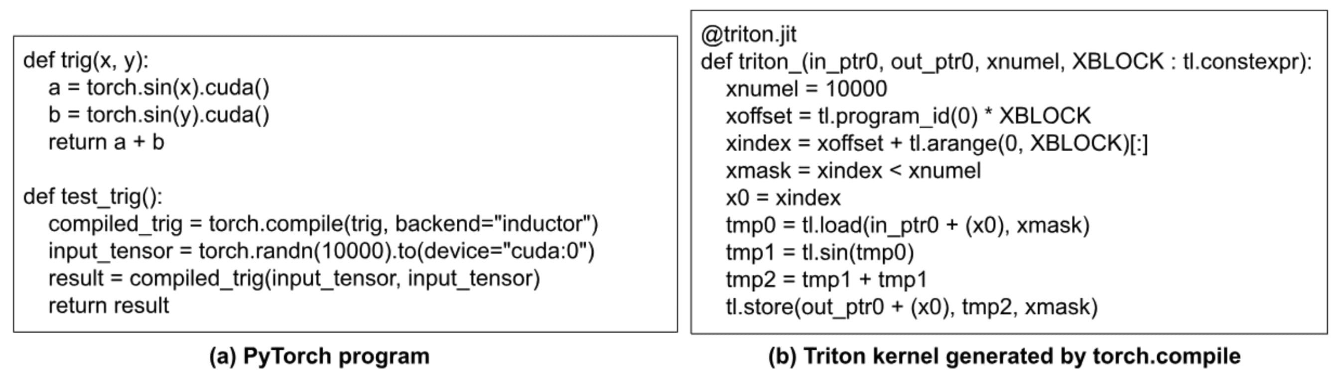
Fig. 1: How PT2 improves performance with fusion and dead-code elimination.

• Reducing the type conversion overhead for using lower-precision data types:
  • PyTorch 1.x supports Automatic Mixed Precision (AMP). While AMP can reduce the compute time of an op, it introduces type conversion overhead before and after the op. PT2 can increase AMP performance by optimizing away unnecessary type conversion code, significantly reducing its overhead. As an example, Figure 2(a) converts three 32-bit input tensors (a32, b32, c32) to bf16 before doing the matrix multiplications. Nevertheless, in this example, a32 and c32 are actually the same tensor (a_float32). So, there is no need to convert a_float32 twice, as shown in the code generated by torch.compile in Figure 2(b). Note that while both this example and the previous one optimize away redundant computations, they are different in the sense that the type conversion code in this example is implicit via torch.autocast, unlike in the previous example where the torch.sin(x).cuda() is explicit in user code.

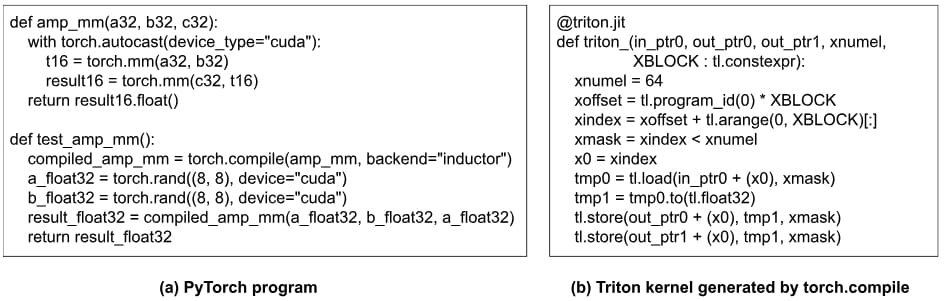
Fig. 2: How PT2 reduces type conversion overhead when using AMP.

• Reusing buffers on the GPU:
  • With a global view, the scheduler in torch.compile can reuse buffers on the GPU, thereby reducing both memory allocation time and memory consumption. Figure 3 shows the driver program that calls the Triton kernels generated for the program in Figure 2(a). We can see that buf1 is reused as buf4.

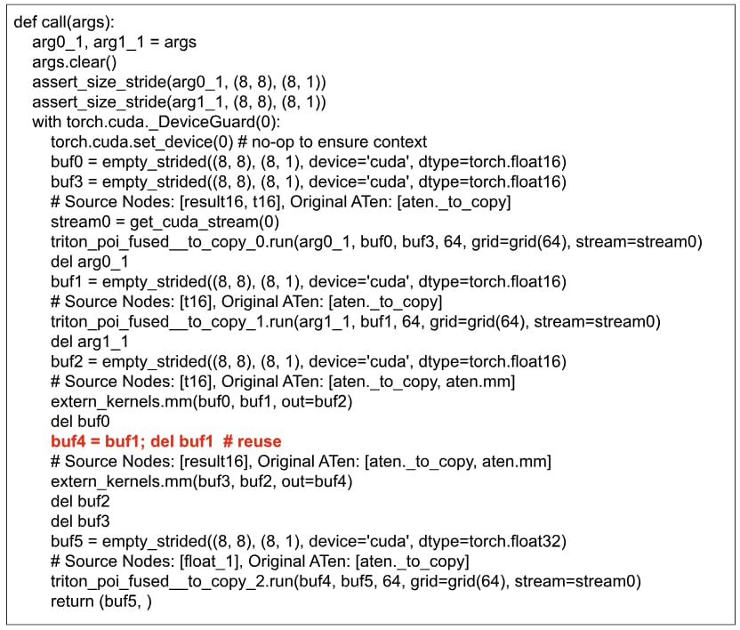
Fig. 3: Reuse of buffers.

• Autotuning:
  • PT2 has options to enable autotuning (via Triton) on matrix-multiply ops, pointwise ops, and reduction ops. Tunable parameters include block size, number of stages, and number of warps. With autotuning, the most performant implementation of an op can be found empirically.

3. Production environment considerations

In this section, we describe a number of important considerations in applying PT2 to production.

3.1 Ensuring no model quality degradation with torch.compile

Applying torch.compile to a model will cause numerical changes because of (1) reordering of floating-point ops during various optimizations such as fusion and (2) use of lower precision data types like bf16 if AMP is enabled. Therefore 100% bitwise compatibility with PT 1.x is not expected. Nevertheless, we still need to make sure that the model quality (measured in some form of numeric scores) is preserved after applying torch.compile. Typically, each production model will have its own range of acceptable scores (e.g., percentage change must be within 0.01%).

In case of a model-quality drop caused by torch.compile, we need to do a deep-dive debug.

One useful technique for debugging a torch.compile-related numeric issue is to apply torch.compile with different backends, in particular “eager” and “aot_eager”, in addition to “inductor”:

• If the numeric issue happens with the “eager” backend, then the forward graph constructed by torch.compile is likely incorrect;
• If the numeric issue doesn’t happen with “eager” but happens with “aot_eager”, then the backward graph constructed by torch.compile is likely incorrect;
• If the numeric issue doesn’t happen with either “eager” or “aot_eager” but happens with “inductor”, then the code generation inside the inductor is likely incorrect.

3.2 Autotuning in production

By default, the autotuning in torch.inductor is done online _while the model is executed. For some production models, we find that the autotuning time can take several hours, which is not acceptable for production. Therefore, we add _offline autotuning which works as depicted in Figure 4. The very first time that a model is run, the details (e.g., input tensor shape, data type etc) on all ops that require tuning will be logged to a database. Then, a tuning process for these ops is run overnight to search for the most performant implementation of each op; the search result is updated to a persistent cache (implemented as a source file of torch.inductor). Next time when the model is run again, the tuned implementation of each op will be found in the cache and chosen for execution.

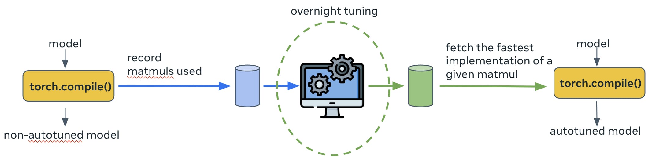
Fig. 4: The offline autotuning used in production.

As we previously discussed in this blog, a profiler is essential for debugging the performance of production models. We have enhanced the profiler to display torch.compile related events on the timeline. The most useful ones are marking which parts of the model are running compiled code so that we can quickly validate if the parts of the model that are supposed to be compiled are actually compiled by torch.compile. For example, the trace in Figure 5 has two compiled regions (with the label “CompiledFunction”). Other useful events are time spent on the compilation and that spent on accessing the compiler’s code-cache.

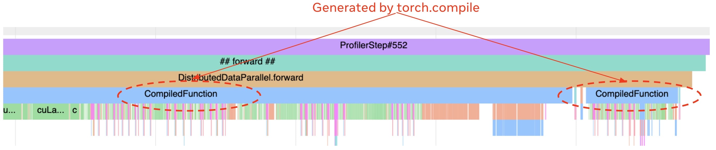
Fig. 5: A trace with two compiled regions.

3.4 Controlling just-in-time compilation time

torch.compile uses just-in-time compilation. The compilation happens when the first batch of data is trained. In our production setting, there is an upper limit on how much time is allowed for a training job to reach its first batch, aka Time-To-First-Batch (TTFB). We need to make sure that enabling torch.compile will not increase TTFB to over the limit. This could be challenging because production models are large and~~ ~~torch.compile can take substantial compilation time. We enable parallel compilation to keep the compile time under control (this is controlled by the global variable compile_threads inside torch/_inductor/config.py, which is already set to the CPU count on OSS Linux). A model is decomposed into one or more computational graphs; each graph is decomposed into multiple Triton kernels. If parallel compilation is enabled, all the Triton kernels in the same graph can be compiled simultaneously (nevertheless, kernels from different graphs are still compiled in serial). Figure 6 illustrates how parallel compilation helps.

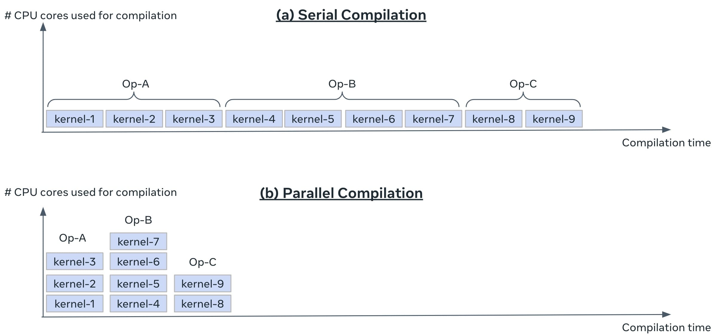
Fig. 6: Using parallel compilation in production.

4. Results

In this section, we use three production models to evaluate PT2. First we show the training time speedups with PT2, using different optimization configs. Second, we show the importance of parallel compilation on the compilation time.

4.1 Training-time speedup with torch.compile

Figure 7 reports the training-time speedup with PT2. For each model, we show four cases: (i) no-compile with bf16, (ii) compile with fp32, (iii) compile with bf16, (iv) compile with bf16 and autotuning. The y-axis is the speedup over the baseline, which is no-compile with fp32. Note that no-compile with bf16 is actually slower than no-compile with fp32, due to the type conversion overhead. In contrast, compiling with bf16 achieves much larger speedups by reducing much of this overhead. Overall, given that these models are already heavily optimized by hand, we are excited to see that torch.compile can still provide 1.14-1.24x speedup.

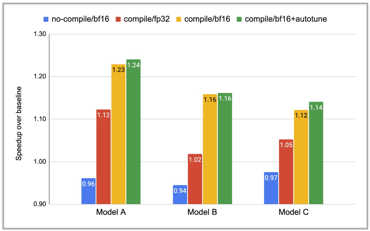
Fig. 7: Training-time speedup with torch.compile (note: the baseline, no-compile/fp32, is_ omitted _in this figure).

4.2 Compilation-time reduction with parallel compilation

Figure 8 shows the compilation time with and without parallel compilation. While there is still room for improvement on the serial compilation time, parallel compilation has reduced the compilation overhead on TTFB to an acceptable level. Models B and C benefit more from parallel compilation than Model A does because they have more distinct Triton kernels per graph.

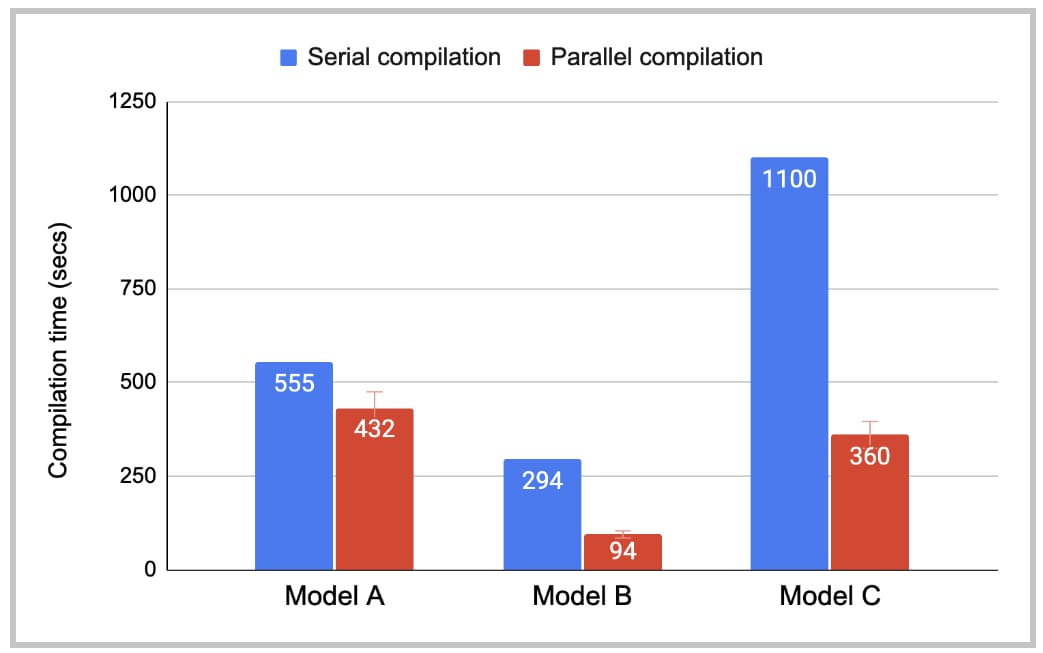
Fig. 8: PT2 compilation time.

5. Concluding Remarks

In this blog, we demonstrate that PT2 can significantly accelerate the training of large and complex production AI models with reasonable compilation time. In our next blog, we will discuss how PT2 can do general graph transformations.

6. Acknowledgements

Many thanks to Mark Saroufim, Adnan Aziz, and Gregory Chanan for their detailed and insightful reviews.

Read More