Introduction
Ease of use, expressivity, and debuggability are among the core principles of PyTorch. One of the key drivers for the ease of use is that PyTorch execution is by default “eager, i.e. op by op execution preserves the imperative nature of the program. However, eager execution does not offer the compiler based optimization, for example, the optimizations when the computation can be expressed as a graph.
LazyTensor [1], first introduced with PyTorch/XLA, helps combine these seemingly disparate approaches. While PyTorch eager execution is widely used, intuitive, and well understood, lazy execution is not as prevalent yet.
In this post we will explore some of the basic concepts of the LazyTensor System with the goal of applying these concepts to understand and debug performance of LazyTensor based implementations in PyTorch. Although we will use PyTorch/XLA on Cloud TPU as the vehicle for exploring these concepts, we hope that these ideas will be useful to understand other system(s) built on LazyTensors.
LazyTensor
Any operation performed on a PyTorch tensor is by default dispatched as a kernel or a composition of kernels to the underlying hardware. These kernels are executed asynchronously on the underlying hardware. The program execution is not blocked until the value of a tensor is fetched. This approach scales extremely well with massively parallel programmed hardware such as GPUs.
The starting point of a LazyTensor system is a custom tensor type. In PyTorch/XLA, this type is called XLA tensor. In contrast to PyTorch’s native tensor type, operations performed on XLA tensors are recorded into an IR graph. Let’s examine an example that sums the product of two tensors:
import torch
import torch_xla
import torch_xla.core.xla_model as xm

dev = xm.xla_device()

x1 = torch.rand((3, 3)).to(dev)
x2 = torch.rand((3, 8)).to(dev)

y1 = torch.einsum('bs,st->bt', x1, x2)
print(torch_xla._XLAC._get_xla_tensors_text([y1]))
You can execute this colab notebook to examine the resulting graph for y1. Notice that no computation has been performed yet.
y1 = y1 + x2
print(torch_xla._XLAC._get_xla_tensors_text([y1]))
The operations will continue until PyTorch/XLA encounters a barrier. This barrier can either be a mark step() api call or any other event which forces the execution of the graph recorded so far.
xm.mark_step()
print(torch_xla._XLAC._get_xla_tensors_text([y1]))
Once the mark_step() is called, the graph is compiled and then executed on TPU, i.e. the tensors have been materialized. Therefore, the graph is now reduced to a single line y1 tensor which holds the result of the computation.
Compile Once, Execute Often
XLA compilation passes offer optimizations (e.g. op-fusion, which reduces HBM pressure by using scratch-pad memory for multiple ops, ref ) and leverages lower level XLA infrastructure to optimally use the underlying hardware. However, there is one caveat, compilation passes are expensive, i.e. can add to the training step time. Therefore, this approach scales well if and only if we can compile once and execute often (compilation cache helps, such that the same graph is not compiled more than once).
In the following example, we create a small computation graph and time the execution:
y1 = torch.rand((3, 8)).to(dev)
def dummy_step() :
  y1 = torch.einsum('bs,st->bt', y1, x)
  xm.mark_step()
  return y1
%timeit dummy_step
The slowest run took 29.74 times longer than the fastest. This could mean that an intermediate result is being cached.
10000000 loops, best of 5: 34.2 ns per loop
You notice that the slowest step is quite longer than the fastest. This is because of the graph compilation overhead which is incurred only once for a given shape of graph, input shape, and output shape. Subsequent steps are faster because no graph compilation is necessary.
This also implies that we expect to see performance cliffs when the “compile once and execute often” assumption breaks. Understanding when this assumption breaks is the key to understanding and optimizing the performance of a LazyTensor system. Let’s examine what triggers the compilation.
Graph Compilation and Execution and LazyTensor Barrier
We saw that the computation graph is compiled and executed when a LazyTensor barrier is encountered. There are three scenarios when the LazyTensor barrier is automatically or manually introduced. The first is the explicit call of mark_step() api as shown in the preceding example. mark_step() is also called implicitly at every step when you wrap your dataloader with MpDeviceLoader (highly recommended to overlap compute and data upload to TPU device). The Optimizer step method of xla_model also allows to implicitly call mark_step (when you set barrier=True).
The second scenario where a barrier is introduced is when PyTorch/XLA finds an op with no mapping (lowering) to equivalent XLA HLO ops. PyTorch has 2000+ operations. Although most of these operations are composite (i.e. can be expressed in terms of other fundamental operations), some of these operations do not have corresponding lowering in XLA.
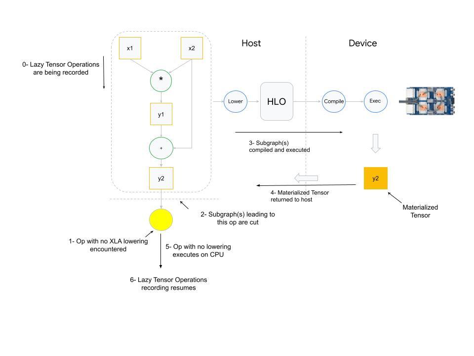
What happens when an op with no XLA lowering is used? PyTorch XLA stops the operation recording and cuts the graph(s) leading to the input(s) of the unlowered op. This cut graph is then compiled and dispatched for execution. The results (materialized tensor) of execution are sent back from device to host, the unlowered op is then executed on the host (cpu), and then downstream LazyTensor operations creating a new graph(s) until a barrier is encountered again.
The third and final scenario which results in a LazyTensor barrier is when there is a control structure/statement or another method which requires the value of a tensor. This statement would at the minimum cause the execution of the computation graph leading to the tensor (if the graph has already been seen) or cause compilation and execution of both.
Other examples of such methods include .item(), isEqual(). In general, any operation that maps Tensor -> Scalar will cause this behavior.
Dynamic Graph
As illustrated in the preceding section, graph compilation cost is amortized if the same shape of the graph is executed many times. It’s because the compiled graph is cached with a hash derived from the graph shape, input shape, and the output shape. If these shapes change it will trigger compilation, and too frequent compilation will result in training time degradation.
Let’s consider the following example:
def dummy_step(x, y, loss, acc=False):
  z = torch.einsum('bs,st->bt', y, x)
  step_loss = z.sum().view(1,)
  if acc:
    loss = torch.cat((loss, step_loss))
  else:
    loss = step_loss
  xm.mark_step()
  return loss


import time
def measure_time(acc=False):
  exec_times = []
  iter_count = 100
  x = torch.rand((512, 8)).to(dev)
  y = torch.rand((512, 512)).to(dev)
  loss = torch.zeros(1).to(dev)
  for i in range(iter_count):
    tic = time.time()
    loss = dummy_step(x, y, loss, acc=acc)
    toc = time.time()
    exec_times.append(toc - tic)
  return exec_times

dyn = measure_time(acc=True) # acc= True Results in dynamic graph
st = measure_time(acc=False) # Static graph, computation shape, inputs and output shapes don't change

import matplotlib.pyplot as plt
plt.plot(st, label = 'static graph')
plt.plot(dyn, label = 'dynamic graph')
plt.legend()
plt.title('Execution time in seconds')
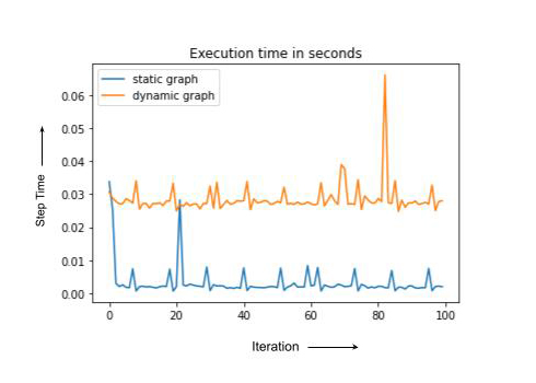
Note that static and dynamic cases have the same computation but dynamic graph compiles every time, leading to the higher overall run-time. In practice, the training step with recompilation can sometimes be an order of magnitude or slower. In the next section we discuss some of the PyTorch/XLA tools to debug training degradation.
Profiling Training Performance with PyTorch/XLA
PyTorch/XLA profiling consists of two major components. First is the client side profiling. This feature is turned on by simply setting the environment variable PT_XLA_DEBUG to 1. Client side profiling points to unlowered ops or device-to-host transfer in your source code. Client side profiling also reports if there are too frequent compilations happening during the training. You can explore some metrics and counters provided by PyTorch/XLA in conjunction with the profiler in this notebook.
The second component offered by PyTorch/XLA profiler is the inline trace annotation. For example:
import torch_xla.debug.profiler as xp

def train_imagenet():
  print('==> Preparing data..')
  img_dim = get_model_property('img_dim')
  ....
  server = xp.start_server(3294)
  def train_loop_fn(loader, epoch):
    ....
    model.train()
    for step, (data, target) in enumerate(loader):
      with xp.StepTrace('Train_Step', step_num=step):
        ....
        if FLAGS.amp:
        ....
        else:
          with xp.Trace('build_graph'):
            output = model(data)
            loss = loss_fn(output, target)
            loss.backward()
          xm.optimizer_step(optimizer)
Notice the start_server api call. The port number that you have used here is the same port number you will use with the tensorboard profiler in order to view the op trace similar to:
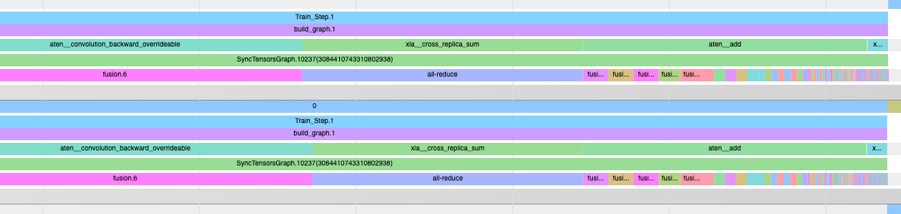
Op trace along with the client-side debugging function is a powerful set of tools to debug and optimize your training performance with PyTorch/XLA. For more detailed instructions on the profiler usage, the reader is encouraged to explore blogs part-1, part-2, and part-3 of the blog series on PyTorch/XLA performance debugging.
Summary
In this article we have reviewed the fundamentals of the LazyTensor system. We built on those fundamentals with PyTorch/XLA to understand the potential causes of training performance degradation. We discussed why “compile once and execute often” helps to get the best performance on LazyTensor systems, and why training slows down when this assumption breaks.
We hope that PyTorch users will find these insights helpful for their novel works with LazyTensor systems.
Acknowledgements
A big thank you to my outstanding colleagues Jack Cao, Milad Mohammedi, Karl Weinmeister, Rajesh Thallam, Jordan Tottan (Google) and Geeta Chauhan (Meta) for their meticulous reviews and feedback. And thanks to the extended PyTorch/XLA development team from Google, Meta, and the open source community to make PyTorch possible on TPUs. And finally, thanks to the authors of the LazyTensor paper not only for developing LazyTensor but also for writing such an accessible paper.