Depending on the quality and complexity of data, data scientists spend between 45–80% of their time on data preparation tasks. This implies that data preparation and cleansing take valuable time away from real data science work. After a machine learning (ML) model is trained with prepared data and readied for deployment, data scientists must often rewrite the data transformations used for preparing data for ML inference. This may stretch the time it takes to deploy a useful model that can inference and score the data from its raw shape and form.
In Part 1 of this series, we demonstrated how Data Wrangler enables a unified data preparation and model training experience with Amazon SageMaker Autopilot in just a few clicks. In this second and final part of this series, we focus on a feature that includes and reuses Amazon SageMaker Data Wrangler transforms, such as missing value imputers, ordinal or one-hot encoders, and more, along with the Autopilot models for ML inference. This feature enables automatic preprocessing of the raw data with the reuse of Data Wrangler feature transforms at the time of inference, further reducing the time required to deploy a trained model to production.
Solution overview
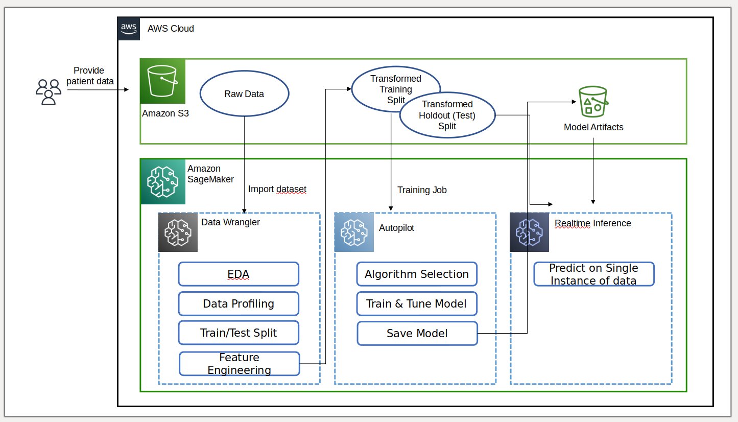
Data Wrangler reduces the time to aggregate and prepare data for ML from weeks to minutes, and Autopilot automatically builds, trains, and tunes the best ML models based on your data. With Autopilot, you still maintain full control and visibility of your data and model. Both services are purpose-built to make ML practitioners more productive and accelerate time to value.
The following diagram illustrates our solution architecture.
Prerequisites
Because this post is the second in a two-part series, make sure you’ve successfully read and implemented Part 1 before continuing.
Export and train the model
In Part 1, after data preparation for ML, we discussed how you can use the integrated experience in Data Wrangler to analyze datasets and easily build high-quality ML models in Autopilot.
This time, we use the Autopilot integration once again to train a model against the same training dataset, but instead of performing bulk inference, we perform real-time inference against an Amazon SageMaker inference endpoint that is created automatically for us.
In addition to the convenience provided by automatic endpoint deployment, we demonstrate how you can also deploy with all the Data Wrangler feature transforms as a SageMaker serial inference pipeline. This enables automatic preprocessing of the raw data with the reuse of Data Wrangler feature transforms at the time of inference.
Note that this feature is currently only supported for Data Wrangler flows that don’t use join, group by, concatenate, and time series transformations.
We can use the new Data Wrangler integration with Autopilot to directly train a model from the Data Wrangler data flow UI.
- Choose the plus sign next to the Scale values node, and choose Train model.
- For Amazon S3 location, specify the Amazon Simple Storage Service (Amazon S3) location where SageMaker exports your data.
If presented with a root bucket path by default, Data Wrangler creates a unique export sub-directory under it—you don’t need to modify this default root path unless you want to.Autopilot uses this location to automatically train a model, saving you time from having to define the output location of the Data Wrangler flow and then define the input location of the Autopilot training data. This makes for a more seamless experience. - Choose Export and train to export the transformed data to Amazon S3.

When export is successful, you’re redirected to the Create an Autopilot experiment page, with the Input data S3 location already filled in for you (it was populated from the results of the previous page). - For Experiment name, enter a name (or keep the default name).
- For Target, choose Outcome as the column you want to predict.
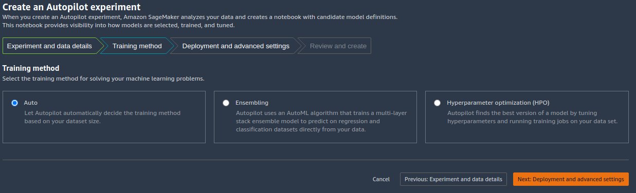
- Choose Next: Training method.

As detailed in the post Amazon SageMaker Autopilot is up to eight times faster with new ensemble training mode powered by AutoGluon, you can either let Autopilot select the training mode automatically based on the dataset size, or select the training mode manually for either ensembling or hyperparameter optimization (HPO).
The details of each option are as follows:
- Auto – Autopilot automatically chooses either ensembling or HPO mode based on your dataset size. If your dataset is larger than 100 MB, Autopilot chooses HPO; otherwise it chooses ensembling.
- Ensembling – Autopilot uses the AutoGluon ensembling technique to train several base models and combines their predictions using model stacking into an optimal predictive model.
- Hyperparameter optimization – Autopilot finds the best version of a model by tuning hyperparameters using the Bayesian optimization technique and running training jobs on your dataset. HPO selects the algorithms most relevant to your dataset and picks the best range of hyperparameters to tune the models.For our example, we leave the default selection of Auto.
- Choose Next: Deployment and advanced settings to continue.
- On the Deployment and advanced settings page, select a deployment option.
It’s important to understand the deployment options in more detail; what we choose will impact whether or not the transforms we made earlier in Data Wrangler will be included in the inference pipeline:- Auto deploy best model with transforms from Data Wrangler – With this deployment option, when you prepare data in Data Wrangler and train a model by invoking Autopilot, the trained model is deployed alongside all the Data Wrangler feature transforms as a SageMaker serial inference pipeline. This enables automatic preprocessing of the raw data with the reuse of Data Wrangler feature transforms at the time of inference. Note that the inference endpoint expects the format of your data to be in the same format as when it’s imported into the Data Wrangler flow.
- Auto deploy best model without transforms from Data Wrangler – This option deploys a real-time endpoint that doesn’t use Data Wrangler transforms. In this case, you need to apply the transforms defined in your Data Wrangler flow to your data prior to inference.
- Do not auto deploy best model – You should use this option when you don’t want to create an inference endpoint at all. It’s useful if you want to generate a best model for later use, such as locally run bulk inference. (This is the deployment option we selected in Part 1 of the series.) Note that when you select this option, the model created (from Autopilot’s best candidate via the SageMaker SDK) includes the Data Wrangler feature transforms as a SageMaker serial inference pipeline.
For this post, we use the Auto deploy best model with transforms from Data Wrangler option.
- For Deployment option, select Auto deploy best model with transforms from Data Wrangler.
- Leave the other settings as default.
- Choose Next: Review and create to continue.
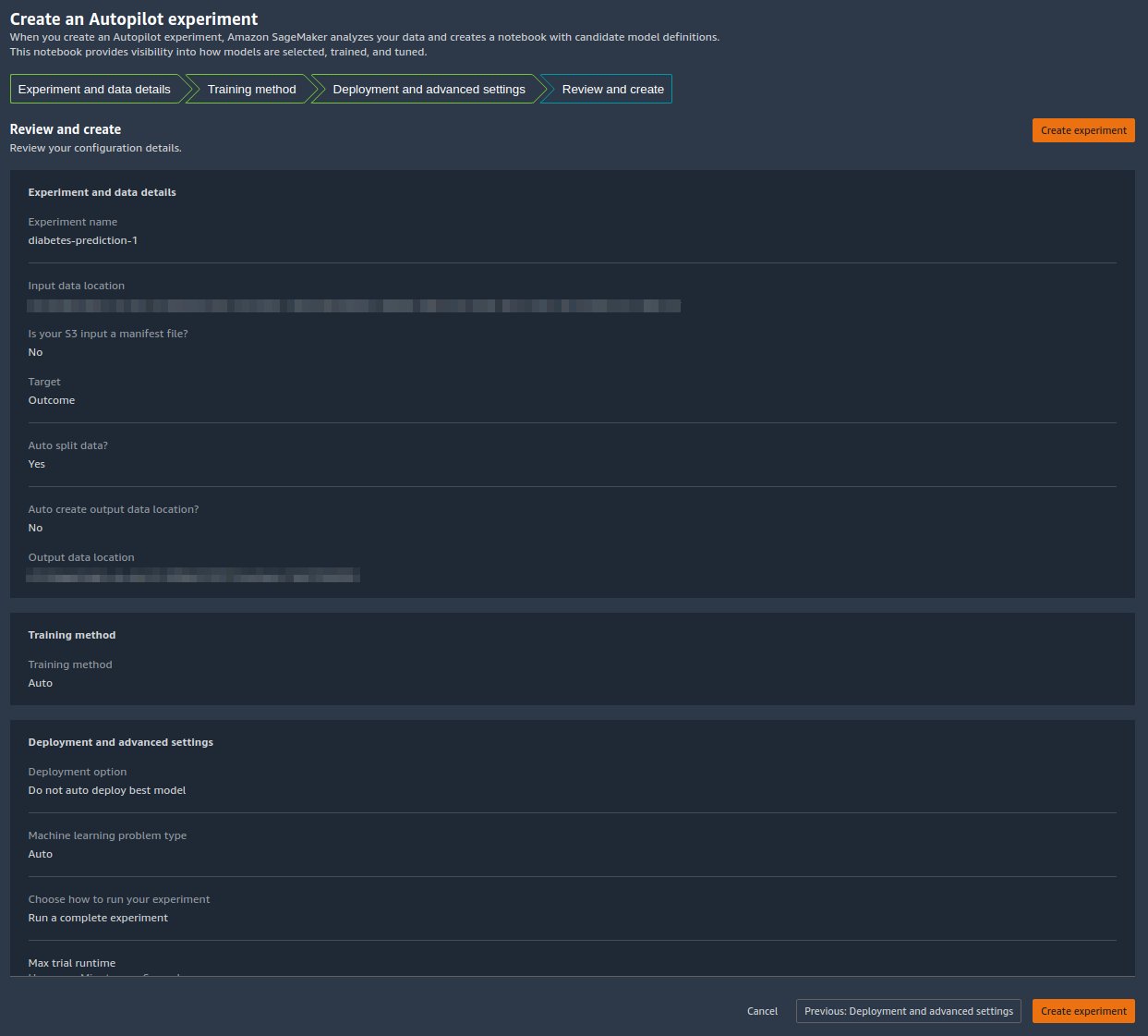
On the Review and create page, we see a summary of the settings chosen for our Autopilot experiment. - Choose Create experiment to begin the model creation process.
You’re redirected to the Autopilot job description page. The models show on the Models tab as they are generated. To confirm that the process is complete, go to the Job Profile tab and look for a Completed value for the Status field.
You can get back to this Autopilot job description page at any time from Amazon SageMaker Studio:
- Choose Experiments and Trials on the SageMaker resources drop-down menu.
- Select the name of the Autopilot job you created.
- Choose (right-click) the experiment and choose Describe AutoML Job.
View the training and deployment
When Autopilot completes the experiment, we can view the training results and explore the best model from the Autopilot job description page.
Choose (right-click) the model labeled Best model, and choose Open in model details.

The Performance tab displays several model measurement tests, including a confusion matrix, the area under the precision/recall curve (AUCPR), and the area under the receiver operating characteristic curve (ROC). These illustrate the overall validation performance of the model, but they don’t tell us if the model will generalize well. We still need to run evaluations on unseen test data to see how accurately the model makes predictions (for this example, we predict if an individual will have diabetes).
Perform inference against the real-time endpoint
Create a new SageMaker notebook to perform real-time inference to assess the model performance. Enter the following code into a notebook to run real-time inference for validation:
After you set up the code to run in your notebook, you need to configure two variables:
endpoint_namepayload_str
Configure endpoint_name
endpoint_name represents the name of the real-time inference endpoint the deployment auto-created for us. Before we set it, we need to find its name.
- Choose Endpoints on the SageMaker resources drop-down menu.
- Locate the name of the endpoint that has the name of the Autopilot job you created with a random string appended to it.
- Choose (right-click) the experiment, and choose Describe Endpoint.

The Endpoint Details page appears. - Highlight the full endpoint name, and press Ctrl+C to copy it the clipboard.

- Enter this value (make sure its quoted) for
endpoint_namein the inference notebook.

Configure payload_str
The notebook comes with a default payload string payload_str that you can use to test your endpoint, but feel free to experiment with different values, such as those from your test dataset.
To pull values from the test dataset, follow the instructions in Part 1 to export the test dataset to Amazon S3. Then on the Amazon S3 console, you can download it and select the rows to use the file from Amazon S3.
Each row in your test dataset has nine columns, with the last column being the outcome value. For this notebook code, make sure you only use a single data row (never a CSV header) for payload_str. Also make sure you only send a payload_str with eight columns, where you have removed the outcome value.
For example, if your test dataset files look like the following code, and we want to perform real-time inference of the first row:
We set payload_str to 10,115,0,0,0,35.3,0.134,29. Note how we omitted the outcome value of 0 at the end.
If by chance the target value of your dataset is not the first or last value, just remove the value with the comma structure intact. For example, assume we’re predicting bar, and our dataset looks like the following code:
In this case, we set payload_str to 85,,20.
When the notebook is run with the properly configured payload_str and endpoint_name values, you get a CSV response back in the format of outcome (0 or 1), confidence (0-1).
Cleaning Up
To make sure you don’t incur tutorial-related charges after completing this tutorial, be sure to shutdown the Data Wrangler app (https://docs.aws.amazon.com/sagemaker/latest/dg/data-wrangler-shut-down.html), as well as all notebook instances used to perform inference tasks. The inference endpoints created via the Auto Pilot deploy should be deleted to prevent additional charges as well.
Conclusion
In this post, we demonstrated how to integrate your data processing, featuring engineering, and model building using Data Wrangler and Autopilot. Building on Part 1 in the series, we highlighted how you can easily train, tune, and deploy a model to a real-time inference endpoint with Autopilot directly from the Data Wrangler user interface. In addition to the convenience provided by automatic endpoint deployment, we demonstrated how you can also deploy with all the Data Wrangler feature transforms as a SageMaker serial inference pipeline, providing for automatic preprocessing of the raw data, with the reuse of Data Wrangler feature transforms at the time of inference.
Low-code and AutoML solutions like Data Wrangler and Autopilot remove the need to have deep coding knowledge to build robust ML models. Get started using Data Wrangler today to experience how easy it is to build ML models using Autopilot.
About the authors
 Geremy Cohen is a Solutions Architect with AWS where he helps customers build cutting-edge, cloud-based solutions. In his spare time, he enjoys short walks on the beach, exploring the bay area with his family, fixing things around the house, breaking things around the house, and BBQing.
 Pradeep Reddy is a Senior Product Manager in the SageMaker Low/No Code ML team, which includes SageMaker Autopilot, SageMaker Automatic Model Tuner. Outside of work, Pradeep enjoys reading, running and geeking out with palm sized computers like raspberry pi, and other home automation tech.
 Dr. John He is a senior software development engineer with Amazon AI, where he focuses on machine learning and distributed computing. He holds a PhD degree from CMU.