Machine learning (ML)-based solutions are capable of solving complex problems, from voice recognition to finding and identifying faces in video clips or photographs. Usually, these solutions use large amounts of training data, which results in a model that processes input data and produces numeric output that can be interpreted as a word, face, or classification category. For many types of problems, this approach works very well.
But what if you have a problem that doesn’t have training data available, or doesn’t fit within the concept of a classification or regression? For example, what if you need to find an optimal ordering for a given set of worker tasks with a given set of conditions and constraints? How do you solve that, especially if the number of tasks is very large?
This post describes genetic algorithms (GAs) and demonstrates how to use them on AWS. GAs are unsupervised ML algorithms used to solve general types of optimization problems, including:
- Optimal data orderings – Examples include creating work schedules, determining the best order to perform a set of tasks, or finding an optimal path through an environment
- Optimal data subsets – Examples include finding the best subset of products to include in a shipment, or determining which financial instruments to include in a portfolio
- Optimal data combinations – Examples include finding an optimal strategy for a task that is composed of many components, where each component is a choice of one of many options
For many optimization problems, the number of potential solutions (good and bad) is very large, so GAs are often considered a type of search algorithm, where the goal is to efficiently search through a huge solution space. GAs are especially advantageous when the fitness landscape is complex and non-convex, so that classical optimization methods such as gradient descent are an ineffective means to find a global solution. Finally, GAs are often referred to as heuristic search algorithms because they don’t guarantee finding the absolute best solution, but they do have a high probability of finding a sufficiently good solution to the problem in a short amount of time.
GAs use concepts from evolution such as survival of the fittest, genetic crossover, and genetic mutation to solve problems. Rather than trying to create a single solution, those evolutionary concepts are applied to a population of different problem solutions, each of which is initially random. The population goes through a number of generations, literally evolving solutions through mechanisms like reproduction (crossover) and mutation. After a number of generations of evolution, the best solution found across all the generations is chosen as the final problem solution.
As a prerequisite to using a GA, you must be able to do the following:
- Represent each potential solution in a data structure.
- Evaluate that data structure and return a numeric fitness score that accurately reflects the solution quality. For example, imagine a fitness score that measures the total time to perform a set of tasks. In that case, the goal would be to minimize that fitness score in order to perform the tasks as quickly as possible.
Each member of the population has a different solution stored in its data structure, so the fitness function must return a score that can be used to compare two candidates against each other. That’s the “survival of the fittest” part of the algorithm—one candidate is evaluated as better than another, and that fitter candidate’s information is passed on to future generations.
One note about terminology: because many of the ideas behind a genetic algorithm come from the field of genetics, the data representation that each member of a population uses is sometimes called a genome. That’s simply another way to refer to the data used to represent a particular solution.
Use case: Finding an optimal route for a delivery van
As an example, let’s say that you work for a company that ships lots of packages all over the world, and your job is focused on the final step, which is delivering a package by truck or van to its final destination.
A given delivery vehicle might have up to 100 packages at the start of a day, so you’d like to calculate the shortest route to deliver all the packages and return the truck to the main warehouse when done. This is a version of a classic optimization problem called The Travelling Salesman Problem, originally formulated in 1930. In the following visualization of the problem, displayed as a top-down map of a section of a city, the warehouse is shown as a yellow dot, and each delivery stop is shown as a red dot.
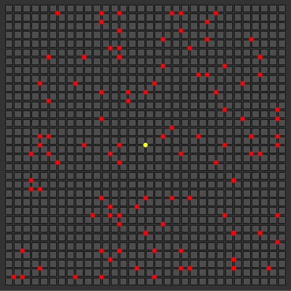
To keep things simple for this demonstration, we assume that when traveling from one delivery stop to another, there are no one-way roads. Due to this assumption, the total distance traveled from one stop to the next is the difference in X coordinates added to the difference in Y coordinates.
If the problem had a slightly different form (like traveling via airplane rather than driving through city streets), we might calculate the distance using the Pythagorean equation, taking the square root of the total of the difference in X coordinates (squared) added to the difference in Y coordinates (squared). For this use case, however, we stick with the total of the difference in X coordinates added to the total of the difference in Y coordinates, because that matches how a truck travels to deliver the packages, assuming two-way streets.
Next, let’s get a sense of how challenging this problem is. In other words, how many possible routes are there with 100 stops where you visit each stop only once? In this case, the math is simple: there are 100 possible first stops multiplied by 99 possible second stops, multiplied by 98 possible third stops, and so on—100 factorial (100!), in other words. That’s 9.3 x 10157 possibilities, which definitely counts as a large solution space and rules out any thoughts of using a brute force approach. After all, with that volume of potential solutions, there really is no way to iterate through all the possible solutions in any reasonable amount of time.
Given that, it seems that a GA could be a good approach for this problem, because GAs are effective at finding good-quality solutions within very large solution spaces. Let’s develop a GA to see how that works.
Representation and a fitness function
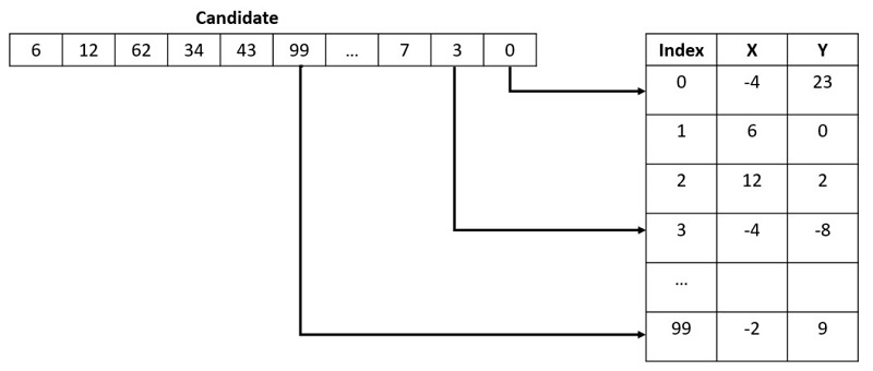
As mentioned earlier, the first step in writing a GA is to determine the data structure for a solution. Suppose that we have a list of all 100 destinations with their associated locations. A useful data representation for this problem is to have each candidate store a list of 100 location indexes that represent the order the delivery van must visit each location. The X and Y coordinates found in the lookup table could be latitude and longitude coordinates or other real-world data.
To implement our package delivery solution, we use a Python script, although almost any modern computer language like Java or C# works well. Open-source packages like inspyred also create the general structure of a GA, allowing you to focus on just the parts that vary from project to project. However, for the purposes of introducing the ideas behind a GA, we write the code without relying on third-party libraries.
As a first step, we represent a potential solution as the following code:
class CandidateSolution(object):
    def __init__(self):
        self.fitness_score = 0
        num_stops = len(delivery_stop_locations) # a list of (X,Y) tuples
        self.path = list(range(num_stops))
        random.shuffle(self.path)
The class has a fitness_score field and a path field. The path is a list of indexes into delivery_stop_locations, which is a list of (X,Y) coordinates for each delivery stop. That list is loaded from a database elsewhere in the code. We also use random.shuffle(), which ensures that each potential solution is a randomly shuffled list of indexes into the delivery_stop_locations list. GAs always start with a population of completely random solutions, and then rely on evolution to home in on the best solution possible.
With this data structure, the fitness function is straightforward. We start at the warehouse, then travel to the first location in our list, then the second location, and so on until we’ve visited all delivery stop locations, and then we return to the warehouse. In the end, the fitness function simply totals up the distance traveled over that entire trip. The goal of this GA is to minimize that distance, so the smaller the fitness score, the better the solution. We use the following the code to implement the fitness function:
def dist(location_a, location_b):
    xdiff = abs(location_a['X'] - location_b['X'])
    ydiff = abs(location_a['Y'] - location_b['Y'])
    return xdiff + ydiff

 def calc_score_for_candidate(candidate):
    # start with the distance from the warehouse to the first stop
    warehouse_location = {'X': STARTING_WAREHOUSE_X, 'Y': STARTING_WAREHOUSE_Y}
    total_distance = dist(warehouse_location, delivery_stop_locations[candidate.path[0]])

    # then travel to each stop
    for i in range(len(candidate.path) - 1):
        total_distance += dist(
            delivery_stop_locations[candidate.path[i]],
            delivery_stop_locations[candidate.path[i + 1]])

    # then travel back to the warehouse
    total_distance += dist(warehouse_location, delivery_stop_locations
[candidate.path[-1]])
    return total_distance
Now that we have a representation and a fitness function, let’s look at the overall flow of a genetic algorithm.
Program flow for a genetic algorithm
When you have a data representation and a fitness function, you’re ready to create the rest of the GA. The standard program flow includes the following pseudocode:
- Generation 0 – Initialize the entire population with completely random solutions.
- Fitness – Calculate the fitness score for each member of the population.
- Completion check – Take one of the following actions:
- If the best fitness score found in the current generation is better than any seen before, save it as a potential solution.
- If you go through a certain number of generations without any improvement (no better solution has been found), then exit this loop, returning the best found to date.
- Elitism – Create a new generation, initially empty. Take a small percentage (like 5%) of the best-scoring candidates from the current generation and copy them unchanged into the new generation.
- Selection and crossover – To populate the remainder of the new generation, repeatedly select two good candidate solutions from the current generation and combine them to form a new child candidate that gets added to the next generation.
- Mutation – On rare occasions (like 2%, for example), mutate a newly created child candidate by randomly perturbing its data.
- Replace the current generation with the next generation and return to step 2.
When the algorithm exits the main loop, the best solution found during that run is used as the problem’s final solution. However, it’s important to realize that because there is so much randomness in a GA—from the initially completely random candidates to randomized selection, crossover, and mutation—each time you run a GA, you almost certainly get a different result. Because of that randomness, a best practice when using a GA is to run it multiple times to solve the same problem, keeping the very best solutions found across all the runs.
Using a genetic algorithm on AWS via Amazon SageMaker Processing
Due to the inherent randomness that comes with a GA, it’s usually a good idea to run the code multiple times, using the best result found across those runs. This can be accomplished using Amazon SageMaker Processing, which is an Amazon SageMaker managed service for running data processing workloads. In this case, we use it to launch the GA so that multiple instances of the code run in parallel.
Before we start, we need to set up a couple of AWS resources that our project needs, like database tables to store the delivery stop locations and GA results, and an AWS Identity and Access Management (IAM) role to run the GA. Use the AWS CloudFormation template included in the associated GitHub repo to create these resources, and make a note of the resulting ARN of the IAM role. Detailed instructions are included in the README file found in the GitHub repo.
After you create the required resources, populate the Amazon DynamoDB table DeliveryStops (indicating the coordinates for each delivery stop) using the Python script create_delivery_stops.py, which is included in the code repo. You can run this code from a SageMaker notebook or directly from a desktop computer, assuming you have Python and Boto3 installed. See the README in the repo for detailed instructions on running this code.
We use DynamoDB for storing the delivery stops and the results. DynamoDB is a reasonable choice for this use case because it’s highly scalable and reliable, and doesn’t require any maintenance due to it being a fully managed service. DynamoDB can handle more than 10 trillion requests per day and can support peaks of more than 20 million requests per second, although this use case doesn’t require anywhere near that kind of volume.
After you create the IAM role and DynamoDB tables, we’re ready to set up the GA code and run it using SageMaker.
- To start, create a notebook in SageMaker.
Be sure to use a notebook instance rather than SageMaker Studio, because we need a kernel with Docker installed.
To use SageMaker Processing, we first need to create a Docker image that we use to provide a runtime environment for the GA.
- Upload
Dockerfileandgenetic_algorithm.pyfrom the code repo into the root folder for your Jupyter notebook instance. - Open
Dockerfileand ensure that theENV AWS_DEFAULT_REGIONline refers to the AWS Region that you’re using.
The default Region in the file from the repo is us-east-2, but you can use any Region you wish.
- Create a cell in your notebook and enter the following code:
import boto3

print("Building container...")

region = boto3.session.Session().region_name
account_id = boto3.client('sts').get_caller_identity().get('Account')
ecr_repository = 'sagemaker-processing-container-for-ga'
tag = ':latest'
base_uri = '{}.dkr.ecr.{}.amazonaws.com'.format(account_id, region)
repo_uri = '{}/{}'.format(base_uri, ecr_repository + tag)

# Create ECR repository and push docker image
!docker build -t $ecr_repository docker
!aws ecr get-login-password --region $region | docker login --username AWS --password-stdin $base_uri
!aws ecr create-repository --repository-name $ecr_repository
!docker tag {ecr_repository + tag} $repo_uri
!docker push $repo_uri

print("Container Build done")

iam_role = 'ARN_FOR_THE_IAM_ROLE_CREATED_EARLIER'
Be sure to fill in the iam_role ARN, which is displayed on the Outputs page of the CloudFormation stack that you created earlier. You can also change the name of the Docker image if you wish, although the default value of sagemaker-processing-container-for-ga is reasonable.
Running that cell creates a Docker image that supports Python with the Boto3 package installed, and then registers it with Amazon Elastic Container Registry (Amazon ECR), which is a fully-managed Docker registry that handles everything required to scale or manage the storage of Docker images.
Add a new cell to your notebook and enter and run the following code:
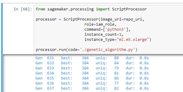
from sagemaker.processing import ScriptProcessor

processor = ScriptProcessor(image_uri=repo_uri,
     role=iam_role,
     command=['python3']
     instance_count=1,
     instance_type="ml.m5.xlarge")

processor.run(code='./genetic_algorithm.py')
This image shows the job launched, and the results displayed below as the GA does its processing:
The ScriptProcessor class is used to create a container that the GA code runs in. We don’t include the code for the GA in the container itself because the ScriptProcessor class is designed to be used as a generic container (preloaded with all required software packages), and the run command chooses a Python file to run within that container. Although the GA Python code is located on your notebook instance, SageMaker Processing copies it to an Amazon Simple Storage Service (Amazon S3) bucket in your account so that it can be referenced by the processing job. Because of that, the IAM role we use must include a read-only permission policy for Amazon S3, along with other required permissions related to services like DynamoDB and Amazon ECR.
Calculating fitness scores is something that can and should be done in parallel, because fitness calculations tend to be fairly slow and each candidate solution is independent of all other candidate solutions. The GA code for this demonstration uses multiprocessing to calculate multiple fitness scores at the same time, which dramatically increases the speed at which the GA runs. We also specify the instance type in the ScriptProcessor constructor. In this case, we chose ml.m5.xlarge in order to use a processor with 4 vCPUs. Choosing an instance type with more vCPUs results in faster runs of each run of the GA, at a higher price per hour. There is no benefit to using an instance type with GPUs for a GA, because all of the work is done via a CPU.
Finally, the ScriptProcessor constructor also specifies the number of instances to run. If you specify a number of instances greater than 1, the same code runs in parallel, which is exactly what we want for a GA. Each instance is a complete run of the GA, run in its own container. Because each instance is completely self-contained, we can run multiple instances at once, and each instance does its calculations and writes its results into the DynamoDB results table.
To review, we’re using two different forms of parallelism for the GA: one is through running multiple instances at once (one per container), and the other is through having each container instance use multiprocessing in order to effectively calculate fitness scores for multiple candidates at the same time.
The following diagram illustrates the overall architecture of this approach.
 The Docker image defines the runtime environment, which is stored in Amazon ECR. That image is combined with a Python script that runs the GA, and SageMaker Processing uses one or more containers to run the code. Each instance reads configuration data from DynamoDB and writes results into DynamoDB.
Genetic operations
Now that we know how to run a GA using SageMaker, let’s dive a little deeper into how we can apply a GA to our delivery problem.
Selection
When we select two parents for crossover, we want a balance between good quality and randomness, which can be thought of as genetic diversity. If we only pick candidates with the best fitness scores, we miss candidates that have elements that might eventually help find a great solution, even though the candidate’s current fitness score isn’t the best. On the other hand, if we completely ignore quality when selecting parents, the evolutionary process doesn’t work very well—we’re ignoring survival of the fittest.
There are a number of approaches for selection, but the simplest is called tournament selection. With a tournament of size 2, you randomly select two candidates from the population and keep the best one. The same applies to a tournament of size 3 or more—you simply use the one with the best fitness score. The larger the number you use, the better quality candidate you get, but at a cost of reduced genetic diversity.
The following code shows the implementation of tournament selection:
def tourney_select(population):
    selected = random.sample(population, TOURNEY_SIZE)
    best = min(selected, key=lambda c: c.fitness_score)
    return best

def select_parents(population):
    # using Tourney selection, get two candidates and make sure they're distinct
    while True:
        candidate1 = tourney_select(population)
        candidate2 = tourney_select(population)
        if candidate1 != candidate2:
            break
    return candidate1, candidate2
Crossover
After we select two candidates, how can we combine them to form one or two children? If both parents are simply lists of numbers and we can’t duplicate or leave out any numbers from the list, combining the two can be challenging.
One approach is called partially mapped crossover. It works as follows:
- Copy each parent, creating two children.
- Randomly select a starting and ending point for crossover within the genome. We use the same starting and ending points for both children.
- For each child, iterate from the starting crossover point to the ending crossover point and perform the following actions on each gene in the child at the current point:
- Find the corresponding gene in the other parent (the one that wasn’t copied into the current child), using the same crossover point. If that gene matches what’s already in the child at that point, continue to the next point, because no crossover is required for the gene.
- Otherwise, find the gene from the alternate parent and swap it with the current gene within the child.
The following diagram illustrates the first step, making copies of both parents.
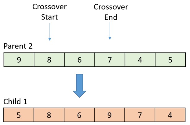
 Each child is crossed over with the alternate parent. The following diagram shows the randomly selected start and end points, with the thick arrow indicating which gene is crossed over next.
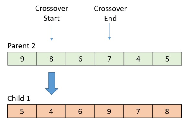
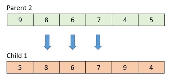
In the first swap position, the parent contributes the value 8. Because the current gene value in the child is 4, the 4 and 8 are swapped within the child.
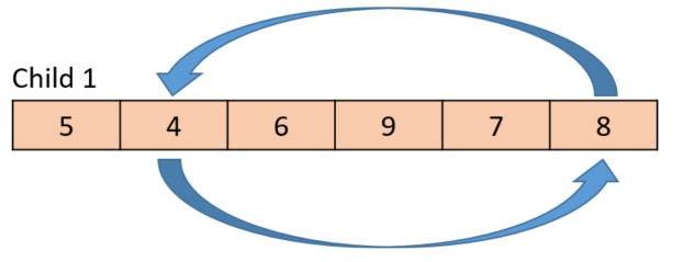
That swap has the effect of taking the gene with value 8 from the parent and placing it within the child at the corresponding position. When the swap is complete, the large arrow moves to the next gene to cross over.
At this point, the sequence is repeated. In this case, both gene values in the current position are the same (6), so the crossover position advances to the next position.
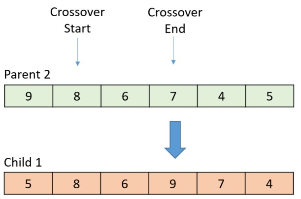
The gene value from the parent is 7 in this case, so the swap occurs within the child.
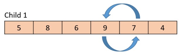
The following diagram shows the final result, with the arrows indicating how the genes were crossed over.
Crossover isn’t a mandatory step, and most GAs use a crossover rate parameter to control how often crossover happens. If two parents are selected but crossover isn’t used, both parents are copied unchanged into the next generation.
We used the following code for the crossover in this solution:
def crossover_parents_to_create_children(parent_one, parent_two):
    child1 = copy.deepcopy(parent_one)
    child2 = copy.deepcopy(parent_two)

    # sometimes we don't cross over, so use copies of the parents
    if random.random() >= CROSSOVER_RATE:
        return child1, child2

    num_genes = len(parent_one.path)
    start_cross_at = random.randint(0, num_genes - 2)  # pick a point between 0 and the end - 2, so we can cross at least 1 stop
    num_remaining = num_genes - start_cross_at
    end_cross_at = random.randint(num_genes - num_remaining + 1, num_genes - 1)

    for index in range(start_cross_at, end_cross_at + 1):
        child1_stop = child1.path[index]
        child2_stop = child2.path[index]

        # if the same, skip it since there is no crossover needed at this gene
        if child1_stop == child2_stop:
            continue

        # find within child1 and swap
        first_found_at = child1.path.index(child1_stop)
        second_found_at = child1.path.index(child2_stop)
        child1.path[first_found_at], child1.path[second_found_at] = child1.path[second_found_at], child1.path[first_found_at]

        # and the same for the second child
        first_found_at = child2.path.index(child1_stop)
        second_found_at = child2.path.index(child2_stop)
        child2.path[first_found_at], child2.path[second_found_at] = child2.path[second_found_at], child2.path[first_found_at]

    return child1, child2
Mutation
Mutation is a way to add genetic diversity to a GA, which is often desirable. However, too much mutation causes the GA to lose its way, so it’s best to use it in moderation if it’s needed at all.
You can approach mutation for this problem in two different ways: swapping and displacement.
A swap mutation is just what it sounds like—two randomly selected locations (genes) are swapped within a genome (see the following diagram).
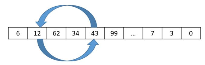
The following code performs the swap:
def swap_mutation(candidate):
    indexes = range(len(candidate.path))
    pos1, pos2 = random.sample(indexes, 2)
    candidate.path[pos1], candidate.path[pos2] = candidate.path[pos2], candidate.path[pos1]
A displacement mutation randomly selects a gene, randomly selects an insertion point, and moves the selected gene into the selected insertion point, shifting other genes as needed to make space (see the following diagram).
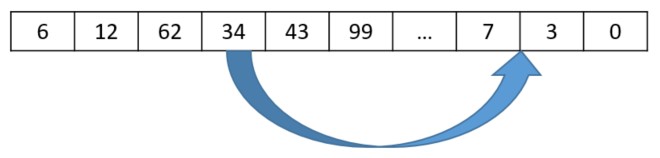
The following code performs the displacement:
def displacement_mutation(candidate):
    num_stops = len(candidate.path)
    stop_to_move = random.randint(0, num_stops - 1)
    insert_at = random.randint(0, num_stops - 1)
    # make sure it's moved to a new index within the path, so it's really different
    while insert_at == stop_to_move:
        insert_at = random.randint(0, num_stops - 1)
    stop_index = candidate.path[stop_to_move]
    del candidate.path[stop_to_move]
    candidate.path.insert(insert_at, stop_index)
Elitism
An optional part of any GA is elitism, which is done when populating a new generation of candidates. When used, elitism copies a certain percentage of the best-scoring candidates from the current generation into the next generation. Elitism is a method for ensuring that the very best candidates always remain in the population. See the following code:
num_elites = int(ELITISM_RATE * POPULATION_SIZE)
current_generation.sort(key=lambda c: c.fitness_score)
next_generation = [current_generation[i] for i in range(num_elites)]
Results
It’s helpful to compare the results from our GA to those from a baseline algorithm. One common non-GA approach to solving this problem is known as the Nearest Neighbor algorithm, which you can apply in this manner:
- Set our current location to be the warehouse.
- While there are unvisited delivery stops, perform the following:
- Find the unvisited delivery stop that is closest to our current location.
- Move to that stop, making it the current location.
- Return to the warehouse.
The following diagrams illustrate the head-to-head results, using varying numbers of stops.
10 Delivery Stops
| Nearest Neighbor Total distance: 142 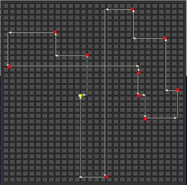 |
Genetic Algorithm Total distance: 124 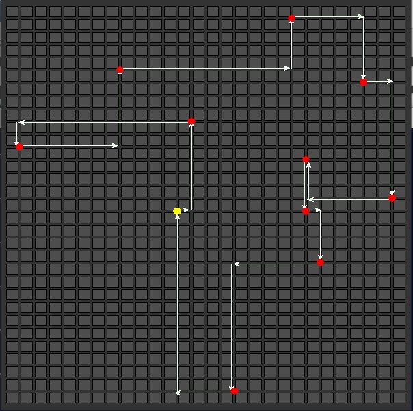 |
25 Delivery Stops
| Nearest Neighbor Total distance: 202 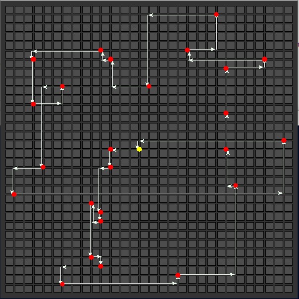 |
Genetic Algorithm Total distance: 170 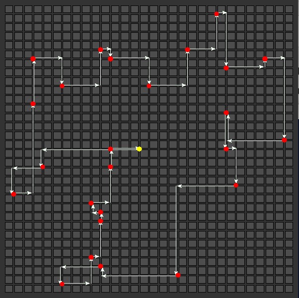 |
50 Delivery Stops
| Nearest Neighbor Total distance: 268 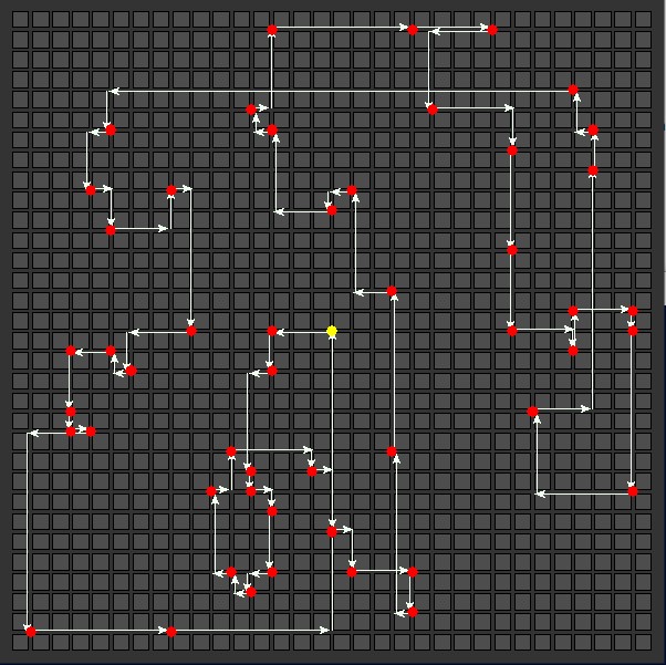 |
Genetic Algorithm Total distance: 252 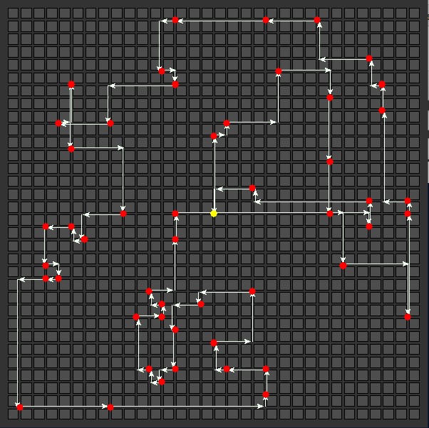 |
75 Delivery Stops
Nearest Neighbor Total distance: 370 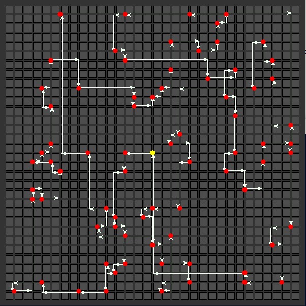 |
Genetic Algorithm Total distance: 318 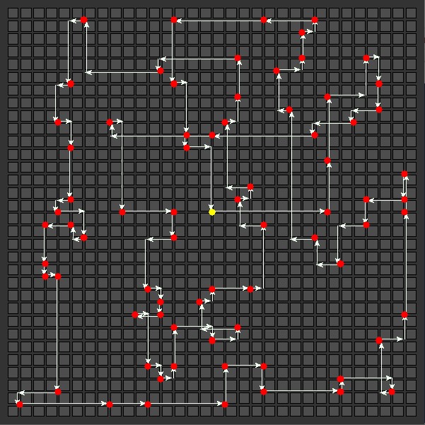 |
100 Delivery Stops
| Nearest Neighbor Total distance: 346 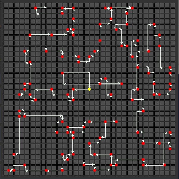 |
Genetic Algorithm Total distance: 368 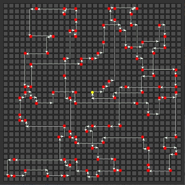 |
The following table summarizes the results.
| # delivery stops | Nearest Neighbor Distance | Genetic Algorithm Distance |
| 10 | 142 | 124 |
| 25 | 202 | 170 |
| 50 | 268 | 252 |
| 75 | 370 | 318 |
| 100 | 346 | 368 |
The Nearest Neighbor algorithm performs well in situations where many locations are clustered tightly together, but can perform poorly when dealing with locations that are more widely distributed. The path calculated for 75 delivery stops is significantly longer than the path calculated for 100 delivery stops—this is an example of how the results can vary widely depending on the data. We need a deeper statistical analysis using a broader set of sample data to thoroughly compare the results of the two algorithms.
On the other hand, for the majority of test cases, the GA solution finds the shorter path, even though it could admittedly be improved with tuning. Like other ML methodologies, genetic algorithms benefit from hyperparameter tuning. The following table summarizes the hyperparameters used in our runs, and we could further tune them to improve the GA’s performance.
| Hyperparameter | Value Used |
| Population size | 5,000 |
| Crossover rate | 50% |
| Mutation rate | 10% |
| Mutation method | 50/50 split between swap and displacement |
| Elitism rate | 10% |
| Tournament size | 2 |
Conclusion and resources
Genetic algorithms are a powerful tool to solve optimization problems, and running them using SageMaker Processing allows you to leverage the power of multiple containers at once. Additionally, you can select instance types that have useful characteristics, like multiple virtual CPUs to optimize running jobs.
If you’d like to learn more about GAs, see Genetic algorithm on Wikipedia, which contains a number of useful links. Although several GA frameworks exist, the code for a GA tends to be relatively simple (because there’s very little math) and you may be able to write the code yourself, or use the accompanying code in our GitHub repo, which includes the CloudFormation template that creates the required AWS infrastructure. Be sure to shut down the CloudFormation stack when you’re done, in order to avoid running up charges.
Although optimization problems are relatively rare compared to other ML applications like classification or regression, when you need to solve one, a genetic algorithm is usually a good option, and SageMaker Processing makes it easy.
About the Author
 Greg Sommerville is a Prototyping Architect on the AWS Envision Engineering Americas Prototyping team, where he helps AWS customers implement innovative solutions to challenging problems with machine learning, IoT and serverless technologies. He lives in Ann Arbor, Michigan and enjoys practicing yoga, catering to his dogs, and playing poker.