Figure 1: Training instability is one of the biggest challenges in training GANs. Despite the existence of successful heuristics like Spectral Normalization (SN) for improving stability, it is poorly-understood why they work. In our research, we theoretically explain why SN stabilizes GAN training. Using these insights, we further propose a better normalization technique for improving GANs’ stability called Bidirectional Scaled Spectral Normalization.
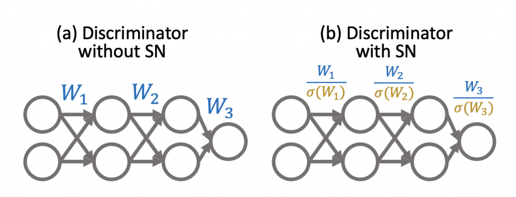
Generative adversarial networks (GANs) are a class of popular generative models enabling many cutting-edge applications such as photorealistic image synthesis. Despite their tremendous success, GANs are notoriously unstable to train—small hyper-parameter changes and even randomness in optimization can cause training to fail altogether, which leads to poor generated samples. One empirical heuristic that is widely used to stabilize GAN training is spectral normalization (SN) (Figure 2). Although it is very widely adopted, little is understood about why it works, and therefore there is little analytical basis for using it, configuring it, and more importantly, improving it.
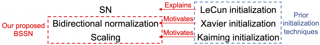
In this post, we discuss our recent work at NeurIPS 2021. We prove that spectral normalization controls two well-known failure modes of training stability: exploding and vanishing gradients. More interestingly, we uncover a surprising connection between spectral normalization and neural network initialization techniques, which not only help explain how spectral normalization stabilizes GANs, but also motivate us to design Bidirectional Scaled Spectral Normalization (BSSN), a simple change to spectral normalization that yields better stability than SN (Figure 3).
Exploding and vanishing gradients cause training instability
Exploding and vanishing gradients describe a problem in which gradients either grow or shrink rapidly during training. It is known in the community that these phenomena are closely related to the instability of GANs. Figure 4 shows an illustrating example: when exploding and vanishing gradients happen, the sample quality measured by inception score (higher is better) deteriorates rapidly.
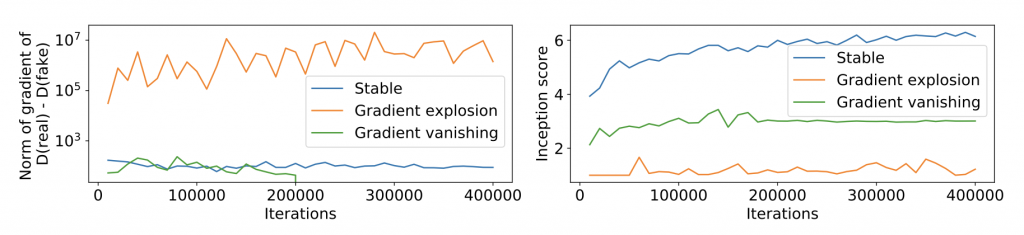
In the next section, we will show how spectral normalization alleviates exploding and vanishing gradients, which may explain its success.
How spectral normalization mitigates exploding gradients
The fact that spectral normalization prevents gradient explosion is not too surprising. Intuitively, it achieves this by limiting the ability of weight tensors to amplify inputs in any direction. More precisely, when the spectral norm of weights = 1 (as ensured by spectral normalization), and the activation functions are 1-Lipschitz (e.g., (Leaky)ReLU), we show that
$$ | text{gradient} |_{text{Frobenius}} leq sqrt{text{number of layers}} cdot | text{input} |.$$
(Please refer to the paper for more general results.) In other words, the gradient norm of spectrally normalized GANs cannot exceed a strict bound. This explains why spectral normalization can mitigate exploding gradients.
Note that this good property is not unique to spectral normalization—our analysis can also be used to show the same result for other normalization and regularization techniques that control the spectral norm of weights, such as weight normalization and orthogonal regularization. The more surprising and important fact is that spectral normalization can also control vanishing gradients at the same time, as discussed below.
How spectral normalization mitigates vanishing gradients
To understand why spectral normalization prevents gradient vanishing, let’s take a brief detour to the world of neural network initialization. In 1996, LeCun, Bottou, Orr, and Müller introduced a new initialization technique (commonly called LeCun initialization) that aimed to prevent vanishing gradients. It achieved this by carefully setting the variance of the weight initialization distribution as $$text{Var}(W)=left(text{fan-in of the layer}right)^{-1},$$ where fan-in of the layer means the number of input connections from the previous layer (e.g., in fully-connected networks, fan-in of the layer is the number of neurons in the previous layer). LeCun et al. showed that
- If the weight variance is larger than ( left(text{fan-in of the layer}right)^{-1} ), the internal outputs of the neural networks could be saturated by bounded activation or loss functions (e.g., sigmoid), which causes vanishing gradients.
- If the weight variance is too small, gradients will also vanish because gradient norms are bounded by the scale of the weights.
We show theoretically that spectral normalization controls the variance of weights in a way similar to LeCun initialization. More specifically, for a weight matrix (Win mathbb{R}^{mtimes n}) with i.i.d. entries from a zero-mean Gaussian distribution (common for weight initialization), we show that
$$ text{Var}left( text{spectrally-normalized } W right) ~~~text{ is on the order of }~~~left( maxleft{ m,n right} right)^{-1} $$
(Please refer to the paper for more general results.) This result has separate implications on the fully-connected layers and convolutional layers:
- For fully-connected layers with a fixed width across hidden layers, (maxleft{m,nright} =m =n =text{fan-in of the layer} ). Therefore, spectrally-normalized weights have exactly the desired variances as LeCun initialization!
- For convolutional layers, the weight (i.e., convolution kernel) is actually a 4-dimensional tensor: ( W in mathbb{R}^{c_{out} c_{in} k_w k_h} ), where (c_{out},c_{in},k_w,k_h) denote the number of output channels, the number of input channels, kernel width, and kernel hight respectively. The popular implementation of spectral normalization normalizes the weights by ( frac{W}{sigmaleft( W_{c_{out} times left(c_{in} k_w k_hright)} right)} ) where (sigmaleft( W_{c_{out} times left(c_{in} k_w k_hright)} right)) is the spectral norm on the reshaped weight, i.e., ( m= c_{out}, n=c_{in} k_w k_h). In hidden layers, usually (maxleft{m,nright} =maxleft{c_{out}, c_{in} k_w k_hright} =c_{in} k_w k_h=text{fan-in of the layer} ). Therefore, spectrally-normalized convolutional layers also maintain the same desired variances as LeCun initialization!
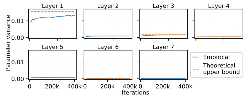
Whereas LeCun initialization only controls the gradient vanishing problem at the beginning of training, we observe empirically that spectral normalization preserves this nice property throughout training (Figure 5). These results may help explain why spectral normalization controls vanishing gradients during GAN training.
How to improve spectral normalization
The next question we ask is: can we use the above theoretical insights to improve spectral normalization? Many advanced initialization techniques have been proposed in recent years to improve LeCun initialization, including Xavier initialization and Kaiming initialization. They derived better parameter variances by incorporating more realistic assumptions into the analysis. We propose Bidirectional Scaled Spectral Normalization (BSSN) so that the parameter variances parallel the ones in these newer initialization techniques:
- Xavier initialization. The idea of Xavier initialization is to set the variance of parameter initialization distribution to be (text{Var}(W)=left(frac{text{fan-in of the layer} + text{fan-out of the layer}}{2}right)^{-1},) which they show to not only control the variances of outputs (as in LeCun initialization), but also the variances of backpropagated gradients, giving better gradient values. We propose Bidirectional Spectral Normalization that normalizes convolutional kernels by (frac{W}{left( sigmaleft(W_{c_{out} times left(c_{in} k_w k_hright)}right) +sigmaleft(W_{c_{in} times left(c_{out} k_w k_hright)}right) right)/2}~~~~~~~). We show that by doing this, the parameter variances mimic the ones in Xavier initialization.
- Kaiming initialization. The analysis in LeCun and Xaiver initialization did not cover activation functions like (Leaky)ReLU which decrease the scales of the network outputs. To cancel out the effect of (Leaky)ReLU, Kaiming initialization scales up the variances in LeCun or Xavier initilization by a constant. Motivated from it, we propose to scale the above normalization formula with a tunable constant (c): (ccdotfrac{W}{left( sigmaleft(W_{c_{out} times left(c_{in} k_w k_hright)}right) +sigmaleft(W_{c_{in} times left(c_{out} k_w k_hright)}right) right)/2}~~~~~~~).
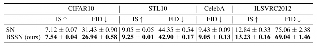
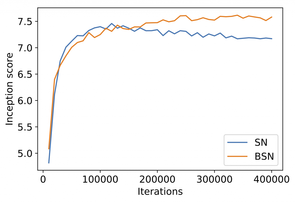
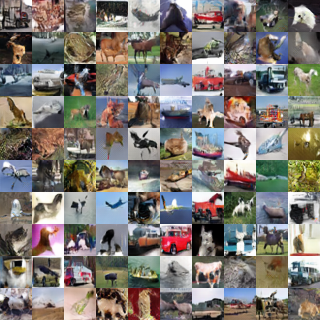
BSSN can be easily plugged into GAN training with minimal code changes and little computational overhead. We compare spectral normalization and BSSN on several image datasets, using standard metrics for image quality like inception score (higher is better) and FID (lower is better). We show that simply replacing spectral normalization with BSSN not only makes GAN training more stable (Figure 6), but also improves sample quality (Table 1). Generated samples from BSSN are in Figure 7.
Links
This post only covers a portion of our theoretical and empirical results. Please refer to our NeurIPS 2021 paper and code if you are interested in learning more.