Fig. 1 We show that learning observation models can be viewed as shaping energy functions that graph optimizers, even non-differentiable ones, optimize. Inference solves for most likely states (x) given model and input measurements (z.) Learning uses training data to update observation model parameters (theta).
Robots perceive the rich world around them through the lens of their sensors. Each sensor observation is a tiny window into the world that provides only a partial, simplified view of reality. To complete their tasks, robots combine multiple readings from sensors into an internal task-specific representation of the world that we call state. This internal picture of the world enables robots to evaluate the consequences of possible actions and eventually achieve their goals. Thus, for successful operations, it is extremely important to map sensor readings into states in an efficient and accurate manner.
Conventionally, the mapping from sensor readings to states relies on models handcrafted by human designers. However, as sensors become more sophisticated and capture novel modalities, constructing such models becomes increasingly difficult. Instead, a more scalable way forward is to convert sensors to tensors and use the power of machine learning to translate sensor readings into efficient representations. This brings up the key question of this post: What is the learning objective? In our recent CoRL paper, LEO: Learning Energy-based Models in Factor Graph Optimization, we propose a conceptually novel approach to mapping sensor readings into states. In that, we learn observation models from data and argue that learning must be done with optimization in the loop.
How does a robot infer states from observations?
Consider a robot hand manipulating an occluded object with only tactile image feedback. The robot never directly sees the object: all it sees is a sequence of tactile images (Lambeta 2020, Yuan 2017). Take a look at any one such image (Fig. 2). Can you tell what the object is and where it might be just from looking at a single image? It seems difficult, right? This is why robots need to fuse information collected from multiple images.
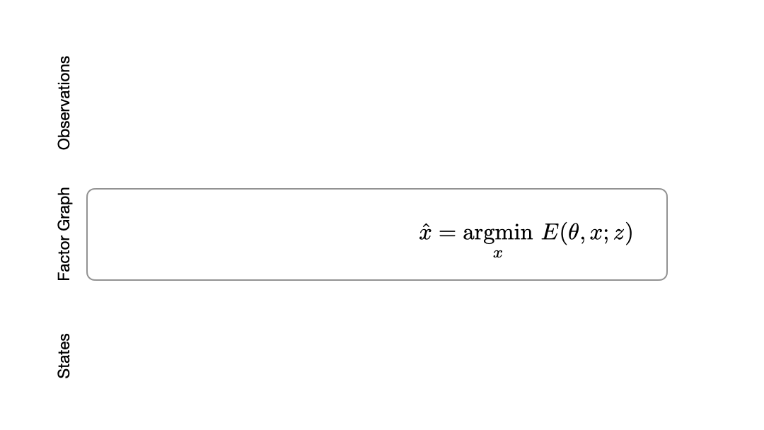
How do we fuse information from multiple observations? A powerful way to do this is by using a factor graph (Dellaert 2017). This approach maintains and dynamically updates a graph where variable nodes are the latent states and edges or factor nodes encode measurements as constraints between variables. Inference solves for the objective of finding the most likely sequence of states given a sequence of observations. Solving for this objective boils down to an optimization problem that can be computed efficiently in an online fashion.
Factor graphs rely on the user specifying an observation model that encodes how likely an observation is given a set of states. The observation model defines the cost landscape that the graph optimizer minimizes. However, in many domains, sensors that produce observations are complex and difficult to model. Instead, we would like to learn the observation model directly from data.
Can we learn observation models from data?
Let’s say we have a dataset of pairs of ground truth state trajectories (x_{gt}) and observations (z). Consider an observation model with learnable parameters (theta) that maps states and observations to a cost. This cost is then minimized by the graph optimizer to get a trajectory (hat{x}). Our objective is to minimize the end-to-end loss (L_{theta}(hat{x},x_{gt})) between the optimized trajectory (hat{x}) and the ground truth (x_{gt}).
What would a typical learning procedure look like? In the forward pass, we have a learned observation model feeding into the graph optimizer to produce an optimized trajectory (hat{x}) (Fig. 3). This is then compared to a ground truth trajectory (x_{gt}) to compute the loss (L_{theta}(.)). The loss is then back-propagated through the inference step to update (theta).
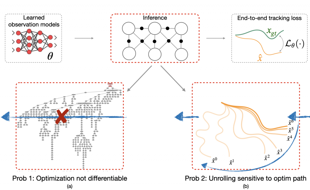
However, there are two problems with this approach. The first problem is that many state-of-the-art optimizers are not natively differentiable. For instance, the iSAM2 graph optimizer (Kaess 2012) used popularly for simultaneous localization and mapping (SLAM) invokes a series of non-differentiable Bayes tree operations and heuristics (Fig. 3a). Secondly, even if one did want to differentiate through the nonlinear optimizer, one would typically do this by unrolling successive optimization steps, and then propagating back gradients through the optimization procedure (Fig. 3b). However, training in this manner can have undesired effects. For example, prior work (Amos 2020) shows instances where even though unrolling gradient descent drives training loss to 0, the resulting cost landscape does not have a minimum on the ground truth. In other words, the learned cost landscape is sensitive to the optimization procedure used during training, e.g., the number of unrolling steps or learning rate.
Learning an energy landscape for the optimizer
We argue that instead of worrying about the optimization procedure, we should only care about the landscape of the energy or cost function that the optimizer has to minimize. We would like to learn an observation model that creates an energy landscape with a global minimum on the ground truth. This is precisely what energy-based models aim to do (LeCun 2006) and that is what we propose in our novel approach LEO that applies ideas from energy-based learning to our problem.
How does LEO work? Let us now demonstrate the inner workings of our approach on a toy example. For this, let us consider a one-dimensional visualization of the energy function represented in Fig 4. We collapse the trajectories down to a single axis. LEO begins by initializing with a random energy function. Note that the ground truth (x_{gt}) is far from the minimum. LEO samples trajectories (hat{x}) around the minimum by invoking the graph optimizer. It then compares these against ground truth trajectories and updates the energy function. The energy-based update rule is simple — push down the cost of ground truth trajectories (x_{gt}) and push up the cost of samples (hat{x}), with the cost of samples effectively acting as a contrastive term. If we keep iterating on this process, the minimum of the energy function eventually centers around the ground truth. At convergence, the gradients of the samples (hat{x}) on average match the gradient of the ground truth trajectory (x_{gt}). Since the samples are over a continuous space of trajectories for which exact computation of the log partition function is intractable, we propose a way to generate such samples efficiently using an incremental Gauss-Newton approximation (Kaess 2012).

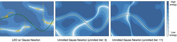
How does LEO perform in practice? Let’s being with a simple regression problem (Amos 2020). We have pairs of ((x,y)) from a ground truth function (y=xsin(x)) and we would like to learn an energy function (E_theta(x,y)) such that (y = {operatorname{argmin}}_{y’} E_theta(x,y’)). LEO begins with a random energy function, but after a few iterations, learns an energy function with a distinct minimum around the ground truth function shown in solid line (Fig. 5). Contrast this to the energy functions learned by unrolling. Not only does it not have a distinct minimum around the ground truth, but it also varies with parameters like the number of unrolling iterations. This is because the learned energy landscape is specific to the optimization procedure used during learning.
Application to Robotics Problems
We evaluate LEO on two distinct robot applications, comparing it to baselines that either learn sequence-to-sequence networks or black-box search methods.
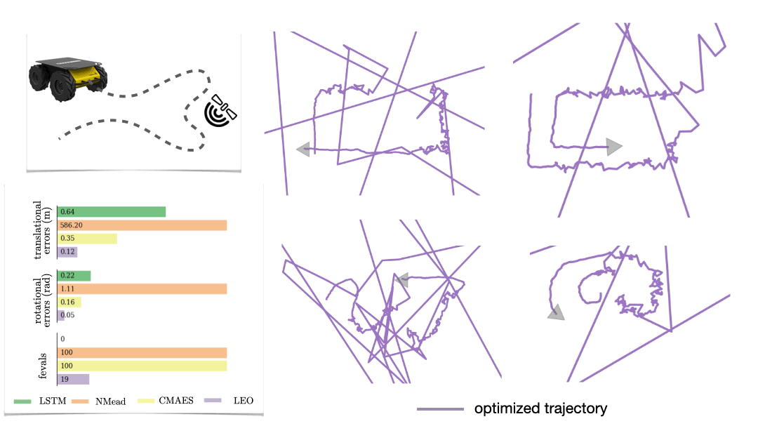
The first is a synthetic navigation task where the goal is to estimate robot poses from odometry and GPS observations. Here we are learning covariances, e.g., how noisy is GPS compared to odometry. Even though LEO is initialized far from the ground truth, it is able to learn parameters that pull the optimized trajectories close to the ground truth (Fig. 6).
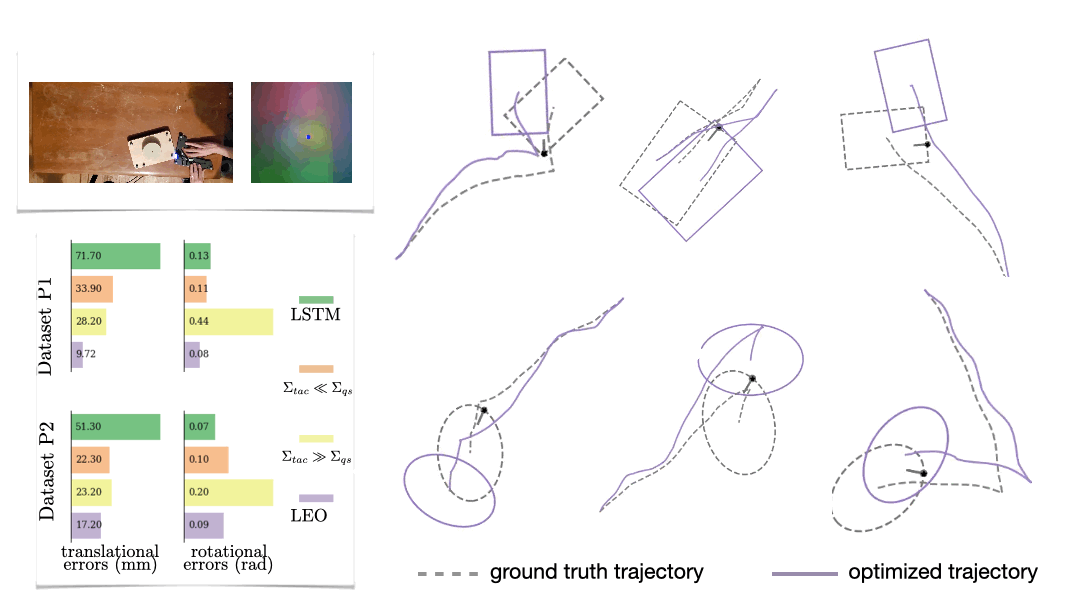
We also look at a real-world manipulation task where an end-effector equipped with a touch sensor is pushing an object (Sodhi 2021). Here we learn a tactile model that maps a pair of tactile images to relative poses used in conjunction with physics and geometric priors. We show that LEO is able to learn parameters that pull optimized trajectories close to the ground truth or various object shapes and pushing trajectories (Fig. 7).
Parting Thoughts
While we focused on learning observation models for perception, the insights on learning energy landscapes for an optimizer extend to other domains such as control and planning. An increasingly unified view of robot perception and control is that both are fundamentally optimization problems. For perception, the objective is to optimize a sequence of states that explain the observations. For control, the objective is to optimize a sequence of actions that accomplish a task.
But what should the objective function be for both of these optimizations? Instead of hand designing observation models for perception or hand designing cost functions for control, we should leverage machine learning to learn these functions from data. To do so easily at scale, it is imperative that we build robotics pipelines and datasets that facilitate learning with optimizers in the loop.
Paper: https://arxiv.org/abs/2108.02274
Code+Video: https://psodhi.github.io/leo
References
[1] Dellaert and Kaess. Factor graphs for robot perception. Foundations and Trends in Robotics, 2017.[2] Kaess et al. iSAM2: Incremental smoothing and mapping using the Bayes tree. Intl. J. of Robotics Research (IJRR), 2012.
[3] LeCun et al. A tutorial on energy-based learning. Predicting structured data, 2006.
[4] Ziebart et al. Maximum entropy inverse reinforcement learning. AAAI Conf. on Artificial Intelligence, 2008.
[5] Amos and Yarats. The differentiable cross-entropy method. International Conference on Machine Learning (ICML), 2020.
[6] Yi et al. Differentiable factor graph optimization for learning smoothers. IEEE/RSJ Intl. Conf. on Intelligent Robots and Systems (IROS), 2021.
[7] Sodhi et al. Learning tactile models for factor graph-based estimation. IEEE Intl. Conf. on Robotics and Automation (ICRA), 2021.
[8] Lambeta et al. DIGIT: A novel design for a low-cost compact high-resolution tactile sensor with application to in-hand manipulation. IEEE Robotics and Automation Letters (RAL), 2020.