Just like the fundamental laws of classical and quantum mechanics taught us how to control and optimize the physical world for engineering purposes, a better understanding of the laws governing neural network learning dynamics can have a profound impact on the optimization of artificial neural networks. This raises a foundational question: what, if anything, can we quantitatively understand about the learning dynamics of state-of-the-art deep learning models driven by real-world datasets?
In order to make headway on this extremely difficult question, existing works have made major simplifying assumptions on the architecture, such as restricting to a single hidden layer 1, linear activation functions 2, or infinite width layers 3. These works have also ignored the complexity introduced by the optimizer through stochastic and discrete updates. In the present work, rather than introducing unrealistic assumptions on the architecture or optimizer, we identify combinations of parameters with simpler dynamics (as shown Fig. 1) that can be solved exactly!
Fig. 1. We plot the per-parameter dynamics (left) and per-filter squared Euclidean norm dynamics (right) for the convolutional layers of a VGG-16 model (with batch normalization) trained on Tiny ImageNet with SGD with learning rate , weight decay , and batch size . Each color represents a different convolutional block. While the parameter dynamics are noisy and chaotic, the neuron dynamics are smooth and patterned.
Symmetries in the loss shape gradient and Hessian geometry
While we commonly initialize neural networks with random weights, their gradients and Hessians at all points in training, no matter the loss or dataset, obey certain geometric constraints. Some of these constraints have been noticed previously as a form of implicit regularization, while others have been leveraged algorithmically in applications from network pruning to interpretability. Remarkably, all these geometric constraints can be understood as consequences of numerous symmetries in the loss introduced by neural network architectures.
A set of parameters observes a symmetry in the loss if the loss doesn’t change under a certain transformation of these parameters. This invariance introduces associated geometric constraints on the gradient and Hessian. We consider three families of symmetries (translation, scale, and rescale) that commonly appear in modern neural network architectures.
- Translation symmetry is defined by the transformation where is the indicator vector for some subset of the parameters . Any network using the softmax function gives rise to translation symmetry for the parameters immediately preceding the function.
- Scale symmetry is defined by the transformation where . Batch normalization leads to scale invariance for the parameters immediately preceding the function.
- Rescale symmetry is defined by the transformation where and are two disjoint sets of parameters. For networks with continuous, homogeneous activation functions (e.g. ReLU, Leaky ReLU, linear), this symmetry emerges at every hidden neuron by considering all incoming and outgoing parameters to the neuron.
These symmetries enforce geometric constraints on the gradient of a neural network ,
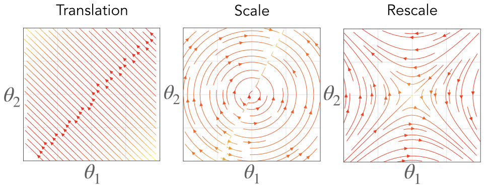
Fig. 2. We visualize the vector fields associated with simple network components that have translation, scale, and rescale symmetry. On the right we consider the vector field associated with a neuron where is the softmax function. In the middle we consider the vector field associated with a neuron where is the batch normalization function. On the left we consider the vector field associated with a linear path .
Symmetry leads to conservation laws under gradient flow
We now consider how geometric constraints on gradients and Hessians, arising as a consequence of symmetry, impact the learning dynamics given by stochastic gradient descent (SGD). We will consider a model parameterized by , a training dataset of size , and a training loss with corresponding gradient . The gradient descent update with learning rate is , which is a forward Euler discretization with step size of the ordinary differential equation (ODE) . In the limit as , gradient descent exactly matches the dynamics of this ODE, which is commonly referred to as gradient flow. Equipped with a continuous model for the learning dynamics, we now ask how do the dynamics interact with the geometric properties introduced by symmetries?
Strikingly similar to Noether’s theorem, which describes a fundamental relationship between symmetry and conservation for physical systems governed by Lagrangian dynamics, every symmetry of a network architecture has a corresponding “conserved quantity” through training under gradient flow. Just as the total kinetic and potential energy is conserved for an idealized spring in harmonic motion, certain combinations of parameters are constant under gradient flow dynamics.
Consider some subset of the parameters that respects either a translation, scale, or rescale symmetry. As discussed earlier, the gradient of the loss is always perpendicular to the vector field that generates the symmetry . Projecting the gradient flow learning dynamics onto the generator vector field yields a differential equation . Integrating this equation through time results in the conservation laws,
Each of these equations define a conserved constant through training, effectively restricting the possible trajectory the parameters take through learning. For parameters with translation symmetry, their sum is conserved, effectively constraining their dynamics to a hyperplane. For parameters with scale symmetry, their Euclidean norm is conserved, effectively constraining their dynamics to a sphere. For parameters with rescale symmetry, their difference in squared Euclidean norm is conserved, effectively constraining their dynamics to a hyperbola.
Fig. 3. Associated with each symmetry is a conserved quantity constraining the gradient flow dynamics to a surface. For translation symmetry (right) the flow is constrained to a hyperplane where the intercept is conserved. For scale symmetry (middle) the flow is constrained to a sphere where the radius is conserved. For rescale symmetry (left) the flow is constrained to a hyperbola where the axes are conserved. The color represents the value of the conserved quantity, where blue is positive and red is negative, and the black lines are level sets.
A realistic continuous model for stochastic gradient descent
While the conservation laws derived with gradient flow are quite striking, empirically we know they are broken, as demonstrated in Fig. 1. Gradient flow is too simple of a continuous model for realistic SGD training, it fails to account for the effect of hyperparameters such as weight decay and momentum, the effect of stochasticity introduced by random batches of data, and the effect of discrete updates due to a finite learning rate. Here, we consider how to address these effects individually to construct more realistic continuous models of SGD.
Modeling weight decay. Explicit regularization through the addition of an penalty on the parameters, with regularization constant , is a very common practice when training neural networks. Weight decay modifies the gradient flow trajectory pulling the network towards the origin in parameter space.
Modeling momentum. Momentum is a common extension to SGD that uses an exponentially moving average of gradients to update parameters rather than a single gradient evaluation. The method introduces an additional hyperparameter , which controls how past gradients are used in future updates, resulting in a form of “inertia” that accelerates the learning dynamics rescaling time, but leaves the gradient flow trajectory intact.
Modeling stochasticity. Stochastic gradients arise when we consider a batch of size drawn uniformly from the indices forming the unbiased gradient estimate . We can model the batch gradient as a noisy version of the true gradient . However, because both the batch gradient and true gradient observe the same geometric properties introduced by symmetry, this noise has a special low-rank structure. In other words, stochasticity introduced by random batches does not affect the gradient flow dynamics in the directions associated with symmetry.
Modeling discretization. Gradient descent always moves in the direction of steepest descent on a loss function at each step, however, due to the finite nature of the learning rate, it fails to remain on the continuous steepest descent path given by gradient flow. In order to model this discrepancy, we borrow tools from the numerical analysis of partial differential equations. In particular, we use modified equation analysis 4, which determines how to model the numerical artifacts introduced by a discretization of a PDE. In our paper we present two methods based on modified equation analysis and recent works 5, 6, which modify gradient flow, with either higher order derivatives of the loss or higher order temporal derivatives of the parameters, to account for the effect of discretization on the learning dynamics.
Fig. 4. We visualize the trajectories of gradient descent with momentum (black dots), gradient flow (blue line), and the modified dynamics (red line) on the quadratic loss . The modified continuous dynamics visually track the discrete dynamics much better than the original gradient flow dynamics.
Combining symmetry and modified gradient flow to derive exact learning dynamics
We now study how weight decay, momentum, stochastic gradients, and finite learning rates all interact to break the conservation laws of gradient flow. Remarkably, even when using a more realistic continuous model for stochastic gradient descent, we can derive exact learning dynamics for the previously conserved quantities. To do this we (i) consider a realistic continuous model for SGD, (ii) project these learning dynamics onto the generator vector fields associated with each symmetry, (iii) harness the geometric constraints introduced by symmetry to derive simplified ODEs, and (iv) solve these ODEs to obtain exact dynamics for the previously conserved quantities. We first consider the continuous model of SGD without momentum incorporating weight decay, stochasticity, and a finite learning rate. In this setting, the exact dynamics for the parameter combinations tied to the symmetries are,
Notice how these equations are equivalent to the conservation laws when . Remarkably, even in typical hyperparameter settings (weight decay, stochastic batches, finite learning rates), these solutions match nearly perfectly with empirical results from modern neural networks (VGG-16) trained on real-world datasets (Tiny ImageNet), as shown in Fig. 5.
Fig. 5. We plot the column sum of the final linear layer (left) and the difference between squared channel norms of the fifth and fourth convolutional layer (right) of a VGG-16 model without batch normalization. We plot the squared channel norm of the second convolution layer (middle) of a VGG-16 model with batch normalization. Both models are trained on Tiny ImageNet with SGD with learning rate , weight decay , batch size , for epochs. Colored lines are empirical and black dashed lines are the theoretical predictions.
Translation dynamics. For parameters with translation symmetry, this equation implies that the sum of these parameters decays exponentially to zero at a rate proportional to the weight decay. In particular, the dynamics do not directly depend on the learning rate nor any information of the dataset due to the lack of curvature in the gradient field for these parameters (as shown in Fig. 2).
Scale dynamics. For parameters with scale symmetry, this equation implies that the norm for these parameters is the sum of an exponentially decaying memory of the norm at initialization and an exponentially weighted integral of gradient norms accumulated through training. Compared to the translation dynamics, the scale dynamics do depend on the data through the gradient norms accumulated throughout training.
Rescale dynamics. For parameters with rescale symmetry, this equation is the sum of an exponentially decaying memory of the difference in norms at initialization and an exponentially weighted integral of difference in gradient norms accumulated through training. Similar to the scale dynamics, the rescale dynamics do depend on the data through the gradient norms, however unlike the scale dynamics we have no guarantee that the integral term is always positive.
Conclusion
Despite being the central guiding principle in the exploration of the physical world, symmetry has been underutilized in understanding the mechanics of neural networks. In this paper, we constructed a unifying theoretical framework harnessing the geometric properties of symmetry and realistic continuous equations for SGD that model weight decay, momentum, stochasticity, and discretization. We use this framework to derive exact dynamics for meaningful combinations of parameters, which we experimentally verified on large scale neural networks and datasets. Overall, our work provides a first step towards understanding the mechanics of learning in neural networks without unrealistic simplifying assumptions.
For more details check out our ICLR paper or this seminar presentation!
Acknowledgments
We would like to thank our collaborator Javier Sagastuy-Brena and advisors Surya Ganguli and Daniel Yamins.
We would also like to thank Megha Srivastava for very helpful feedback on this post.
-
David Saad and Sara Solla. Dynamics of on-line gradient descent learning for multilayer neural networks.Advances in neural information processing systems, 8:302–308, 1995. ↩
-
Andrew M Saxe, James L McClelland, and Surya Ganguli. A mathematical theory of semantic development in deep neural networks. Proc. Natl. Acad. Sci. U. S. A., May 2019. ↩
-
Arthur Jacot, Franck Gabriel, and Clément Hongler. Neural tangent kernel: Convergence and generalization in neural networks. In Advances in neural information processing systems, pp.8571–8580, 2018 ↩
-
RF Warming and BJ Hyett. The modified equation approach to the stability and accuracy analysis of finite-difference methods. Journal of computational physics, 14(2):159–179, 1974. ↩
-
David GT Barrett and Benoit Dherin. Implicit gradient regularization.arXiv preprintarXiv:2009.11162, 2020. ↩
-
Nikola B Kovachki and Andrew M Stuart. Analysis of momentum methods.arXiv preprint arXiv:1906.04285, 2019. ↩