The $20 million program will support projects for three years.Read More
3 questions about the Amazon–NSF collaboration on fairness in AI
NSF deputy assistant director Erwin Gianchandani on the challenges addressed by funded projects.Read More

How-to deploy TensorFlow 2 Models on Cloud AI Platform
Posted by Sara Robinson, Developer Advocate
Google Cloud’s AI Platform recently added support for deploying TensorFlow 2 models. This lets you scalably serve predictions to end users without having to manage your own infrastructure. In this post, I’ll walk you through the process of deploying two different types of TF2 models to AI Platform and use them to generate predictions with the AI Platform Prediction API. I’ll include one example for an image classifier and another for structured data. We’ll start by adding code to existing TensorFlow tutorials, and finish with models deployed on AI Platform. In addition to cloud-based deployment options, TensorFlow also includes open source tools for deploying models, like TensorFlow Serving, which you can run on your own infrastructure. Here, our focus is on using a managed service.
AI Platform supports both autoscaling and manual scaling options. Autoscaling means your model infrastructure will scale to zero when no one is calling your model endpoint so that you aren’t charged when your model isn’t in use. If usage increases, AI Platform will automatically add resources to meet demand. Manual scaling lets you specify the number of nodes you’d like to keep running at all times, which can reduce cold start latency on your model.
The focus here will be on the deployment and prediction processes. AI Platform includes a variety of tools for custom model development, including infrastructure for training and hosted notebooks. When we refer to AI Platform in this post, we’re talking specifically about AI Platform Prediction, a service for deploying and serving custom ML models. In this post, we’ll build on existing tutorials in the TensorFlow docs by adding code to deploy your model to Google Cloud and get predictions.
In order to deploy your models, you’ll need a Google Cloud project with billing activated (you can also use the Google Cloud Platform Free Tier). If you don’t have a project yet, follow the instructions here to create one. Once you’ve created a project, enable the AI Platform API.
Deploying a TF2 image model to AI Platform
To show you how to deploy a TensorFlow 2 model on AI Platform, I’ll be using the model trained in this tutorial from the TF documentation. This trains a model on the Fashion MNIST dataset, which classifies images of articles of clothing into 10 different categories. Start by running through that whole notebook. You can click on the “Run in Google Colab” button at the top of the page to get started. Make sure to save your own copy of the notebook so you don’t lose your progress.
We’ll be using the probability_model created at the end of this notebook, since it outputs classifications in a more human-readable format. The output of probability_model is a 10-element softmax array with the probabilities that the given image belongs to each class. Since it’s a softmax array, all of the elements add up to 1. The highest-confidence classification will be the item of clothing corresponding with the index with the highest value.
In order to connect to your Cloud project, you will next need to authenticate your Colab notebook. Inside the notebook you opened for the Fashion MNIST tutorial, create a code cell:
from google.colab import auth
auth.authenticate_user()
Then run the following, replacing “your-project-id-here” with the ID of the Cloud project you created:
CLOUD_PROJECT = 'your-project-id-here'
BUCKET = 'gs://' + CLOUD_PROJECT + '-tf2-models'
For the next few code snippets, we’ll be using gcloud: the Google Cloud CLI along with gsutil, the CLI for interacting with Google Cloud Storage. Run the line below to configure gcloud with the project you created:
!gcloud config set project $CLOUD_PROJECTIn the next step, we’ll create a Cloud Storage bucket and print our GCS bucket URL. This will be used to store your saved model. You only need to run this cell once:
!gsutil mb $BUCKET
print(BUCKET)
Cloud AI Platform expects our model in TensorFlow 2 SavedModel format. To export our model in this format to the bucket we just created, we can run the following command. The model.save() method accepts a GCS bucket URL. We’ll save our model assets into a fashion-mnist subdirectory:
probability_model.save(BUCKET + '/fashion-mnist', save_format='tf')To verify that this exported to your storage bucket correctly, navigate to your bucket in the Cloud Console (visit storage -> browser). You should see something like this: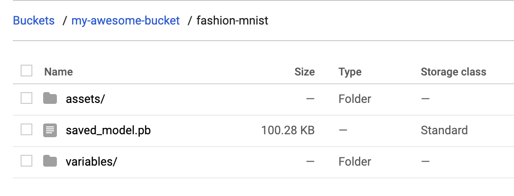
With that we’re ready to deploy the model to AI Platform. In AI Platform, a model resource contains different versions of your model. Model names must be unique within a project. We’ll start by creating a model:
MODEL = 'fashion_mnist'
!gcloud ai-platform models create $MODEL --regions=us-central1
Once this runs, you should see the model in the Models section of the AI Platform Cloud Console:
It has no versions yet, so we’ll create one by pointing AI Platform at the SavedModel assets we uploaded to Google Cloud Storage. Models in AI Platform can have many versions. Versioning can help you ensure that you don’t break users who are dependent on a specific version of your model when you publish a new version. Depending on your use case, you can also serve different model versions to a subset of your users, for example, to run an experiment.
You can create a version either through the Cloud Console UI, gcloud, or the AI Platform API. Let’s deploy our first version with gcloud. First, save some variables that we’ll reference in our deploy command:
VERSION = 'v1'
MODEL_DIR = BUCKET + '/fashion-mnist'
Finally, run this gcloud command to deploy the model:
!gcloud ai-platform versions create $VERSION
  --model $MODEL
  --origin $MODEL_DIR
  --runtime-version=2.1
  --framework='tensorflow'
  --python-version=3.7
This command may take a minute to complete. When your model version is ready, you should see the following in the Cloud Console:
Getting predictions on a deployed image classification model
Now comes the fun part, getting predictions on our deployed model! You can do this with gcloud, the AI Platform API, or directly in the UI. Here we’ll use the API. We’ll use this predict method from the AI Platform docs:
import googleapiclient.discovery

def predict_json(project, model, instances, version=None):

    service = googleapiclient.discovery.build('ml', 'v1')
    name = 'projects/{}/models/{}'.format(project, model)

    if version is not None:
        name += '/versions/{}'.format(version)

    response = service.projects().predict(
        name=name,
        body={'instances': instances}
    ).execute()

    if 'error' in response:
        raise RuntimeError(response['error'])

    return response['predictions']
We’ll start by sending two test images to our model for prediction. To do that, we’ll convert these images from our test set to lists (so it’s valid JSON) and send them to the method we’ve defined above along with our project and model:
test_predictions = predict_json(CLOUD_PROJECT, MODEL, test_images[:2].tolist())In the response, you should see a JSON object with softmax as the key, and a 10-element softmax probability list as the value. We can get the predicted class of the first test image by running:
np.argmax(test_predictions[0]['softmax'])Our model predicts class 9 for this image with 98% confidence. If we look at the beginning of the notebook, we’ll see that 9 corresponds with ankle boot. Let’s plot the image to verify our model predicted correctly. Looks good!
plt.figure()
plt.imshow(test_images[0])
plt.colorbar()
plt.grid(False)
plt.show()
Deploying TensorFlow 2 models with structured data
Now that you know how to deploy an image model, we’ll look at another common model type – a model trained on structured data. Using the same approach as the previous section, we’ll use this tutorial from the TensorFlow docs as a starting point and build upon it for deployment and prediction. This is a binary classification model that predicts whether a patient has heart disease.
To start, make a copy of the tutorial in Colab and run through the cells. Note that this model takes Keras feature columns as input and has two different types of features: numerical and categorical. You can see this by printing out the value of feature_columns. This is the input format our model is expecting, which will come in handy after we deploy it. In addition to sending features as tensors, we can also send them to our deployed model as lists. Note that this model has a mix of numerical and categorical features. One of the categorical features (thal) should be passed in as a string; the rest are either integers or floats.
Following the same process as above, let’s export our model and save it to the same Cloud Storage bucket in a hd-prediction subdirectory:
model.save(BUCKET + '/hd-prediction', save_format='tf')Verify that the model assets were uploaded to your bucket. Since we showed how to deploy models with gcloud in the previous section, here we’ll use the Cloud Console. Start by selecting New Model in the Models section of AI Platform in the Cloud Console:
Then follow these steps (you can see a demo in the following GIF, and you can read about them in the text below).
 |
Head over to the models section of your Cloud console. Then select the New model button and give your model a name, like hd_prediction and select Create.
Once your model resource has been created, select New version. Give it a name (like |
To format our data for prediction, we’ll send each test instance as JSON objects with keys being the name of our features and the values being a list with each feature value. Here’s the code we’ll use to format the first two examples from our test set for prediction:
# First remove the label column
test = test.pop('target')

caip_instances = []
test_vals = test[:2].values

for i in test_vals:
    example_dict = {k: [v] for k,v in zip(test.columns, i)}
    caip_instances.append(example_dict)
Here’s what the resulting array of caip_instances looks like:
[{'age': [60],
  'ca': [2],
  'chol': [293],
  'cp': [4],
  'exang': [0],
  'fbs': [0],
  'oldpeak': [1.2],
  'restecg': [2],
  'sex': [1],
  'slope': [2],
  'thal': ['reversible'],
  'thalach': [170],
  'trestbps': [140]},
...]
We can now call the same predict_json method we defined above, passing it our new model and test instances:
test_predictions = predict_json(CLOUD_PROJECT, 'hd_prediction', caip_instances)Your response will look something like the following (exact numbers will vary):
[{'output_1': [-1.4717596769332886]}, {'output_1': [-0.2714746594429016]}]Note that if you’d like to change the name of the output tensor (currently output_1), you can add a name parameter when you define your Keras model in the tutorial above:
layers.Dense(1, name='prediction_probability')In addition to making predictions with the API, you can also make prediction requests with gcloud. All of the prediction requests we’ve made so far have used online prediction, but AI Platform also supports batch prediction for large offline jobs. To create a batch prediction job, you can make a JSON file of your test instances and kick off the job with gcloud. You can read more about batch prediction here.
What’s next?
You’ve now learned how to deploy two types of TensorFlow 2 models to Cloud AI Platform for scalable prediction. The models we’ve deployed here all use autoscaling, which means they’ll scale down to 0 so you’re only paying when your model is in use. Note that AI Platform also supports manual scaling, which lets you specify the number of nodes you’d like to leave running.
If you’d like to learn more about what we did here, check out the following resources:
- TensorFlow structured data tutorial
- AI Platform Prediction: deploying models guide
- AI Platform Prediction: online prediction guide
I’d love to hear your thoughts on this post. If you’ve got any feedback or topics you’d like to see covered in the future, find me on Twitter at @SRobTweets.
Read More
Sequential Problem Solving by Hierarchical Planning in Latent Spaces
Sequential problem solving is a remarkable ability demonstrated by humans and other intelligent animals. For example, a behavioral ecology study has shown how a crow can plan to retrieve a stone and drop it into the box. This is not an easy task since the stone is initially placed in a cage and the crow cannot get through the bars. But the crow intelligently makes its way to the goal by sequentially picking up a stick, using the stick to reach the stone, and taking the stone to the goal location. In each step, the crow interacts with the environment in a different way which eventually serves the goal of the task. These steps need to be carefully composed together in a specific order, such that the stick will be picked up before being used for reaching the stone.

Can a robot solve sequential problems like this? Imagine if we ask the robot to push a target object to a goal position across a bridge. However, there is an obstacle object on the bridge blocking the way. The robot needs to first remove the obstacle from the bridge and then push the target object to its destination.
Solving such puzzles might seem like a no-brainer to humans, but for robots, to plan in various unseen scenarios is incredibly challenging. To achieve the goal of the task, the robot needs to choose the optimal plan among a plurality of possible solutions. Each plan is composed of a sequence of actions across the time horizon, where at each time step, the robot can take various different actions on different objects. This results in an exponentially growing space of different actions to sample from, which is further complicated by the fact that the robot also needs to predict which actions will be successful solely given the visual observations received by the camera. To find feasible solutions for multi-step manipulation tasks, we would like the robot to generate plans in a structured way and effectively rule out improbable candidates.
To solve these complex sequential problems, we propose CAVIN, a hierarchical planning algorithm. Our algorithm first plans for a sequence of subgoals that lead to task success and then generates actions in the context of the chosen subgoals. To prioritize promising samples, our algorithm learns to capture the distributions of reachable subgoals and feasible actions. The model can be trained with task-agonistic robot interactions and applied to different tasks.
Sampling-based Planning with Deep Generative Models
Even before we know what exactly the goal of the task is, we already know only some actions are useful for forming a promising plan. For example, if the goal is to push a target object to some target position, a push has to be applied onto an object in the first place. If a random action just waves the robot arm around or collides the arm into the table, those actions will either simply not make any progress towards the eventual goal or will violate the constraints of the environment (and hurt our robot!).
Assuming we have a dataset which contains only useful actions, we can learn to capture their distribution using deep generative models, which have been widely used for image and video synthesis. A deep generative model generates a data point given a latent code, which represents the information of the data. To sample an action, we can instead sample the latent code from its prior distribution (e.g. a Gaussian) and use the deep generative model to project it into the action. In this way, our model learns to sample with an emphasis on useful actions.
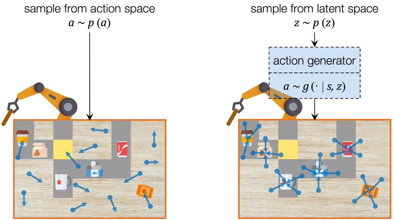
CAVIN: Hierarchical Planning in Learned Latent Spaces
We propose CAVIN to hierarchically generate plans in learned latent spaces. To extend the aforementioned idea of learning to sample for planning with subgoals, we introduce two latent codes, effect code and motion code . Our key insight is to take advantage of the hierarchical structure of the action space, such that the generation of a plan can be factorized into a two-level process:
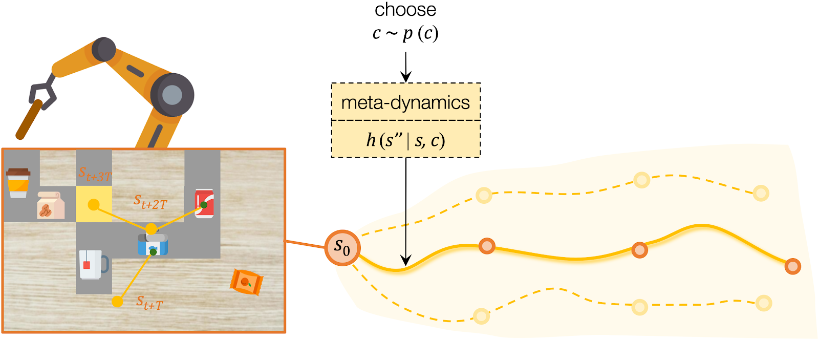
- High-level planning: Selecting the desired effects, in terms of subgoals.
- Low-level planning: Generating detailed actions that lead to the chosen subgoals.
For high-level planning, we sample and select to specify the desired subgoals every steps. Instead of predicting the environment dynamics given a sampled action, here we care about predicting what subgoal can be reached given a sampled . We call this our meta-dynamics model , which captures the distribution of reachable subgoal states
while abstracting away the detailed actions. The meta-dynamics model projects each effect code to a reachable subgoal in the future, conditioned on the current state . We sample and choose the sequence of by predicting the cumulative rewards of each sequence of subgoals.
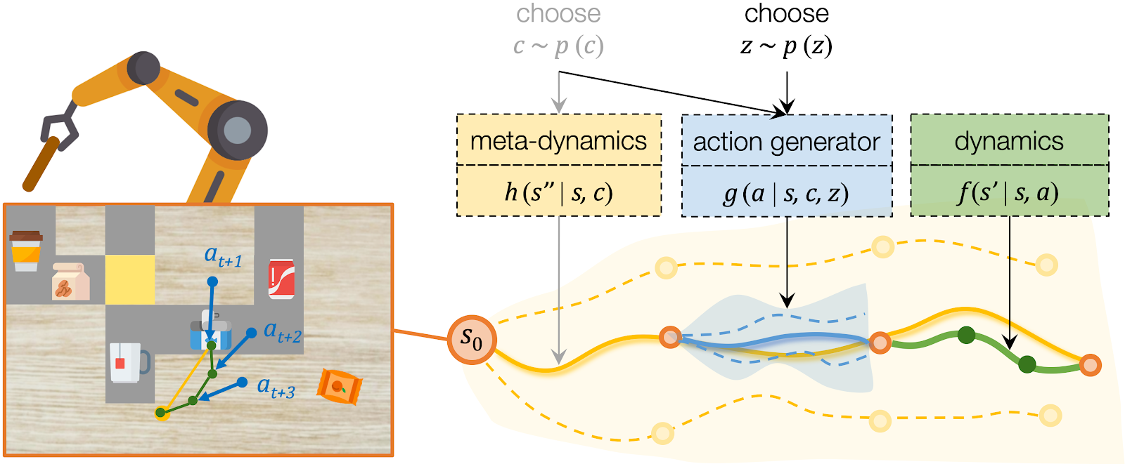
For low-level planning, we sample and select to generate actions that will lead to the subgoals chosen by high-level planning. Action sequences is computed from the desired effect and motion by an action generator . Conditioned on the state and the chosen , the action generator projects into a plausible sequence of that will push the object towards the specified subgoal. The low-level dynamics model evaluates the generated plans by recursively predicting the resulting states . The action sequence which better reaches the subgoals will be executed by the robot.
Learning from Interactions Regardless of Tasks
We assume all tasks are performed in the same environment and the reward functions are provided to the robot as a blackbox function during test time. Therefore CAVIN can be trained in a task-agnostic fashion and later be applied to various task rewards. The data collection is conducted in a physical simulator, where we drop a variety of objects onto the table and ask the robot to randomly push around objects. We only record interesting transitions in the dataset by filtering out those which do not change the object positions or violate constraints.
We propose a cascaded variational inference algorithm to learn the meta-dynamics model and the action generator. Since the latent codes cannot be directly observed, we train the model with a lower bound objective and use two inference networks and , a to infer the latent codes from the collected transitions. To perform hierarchical planning, we need the modules to produce consistent outputs. More specifically, given a chosen , the action sequence generated from any should always yield the subgoal predicted from in the task environment. Therefore, we jointly train the modules and feed the same inferred to both the meta-dynamics model and the action generator.
Experiments
We designed three multi-step manipulation tasks: Clearing, Insertion, and Crossing. All of these tasks share the same table-top workspace and are not seen by the robot during training time. We observe that the robot comes up with diverse strategies in different task scenarios.
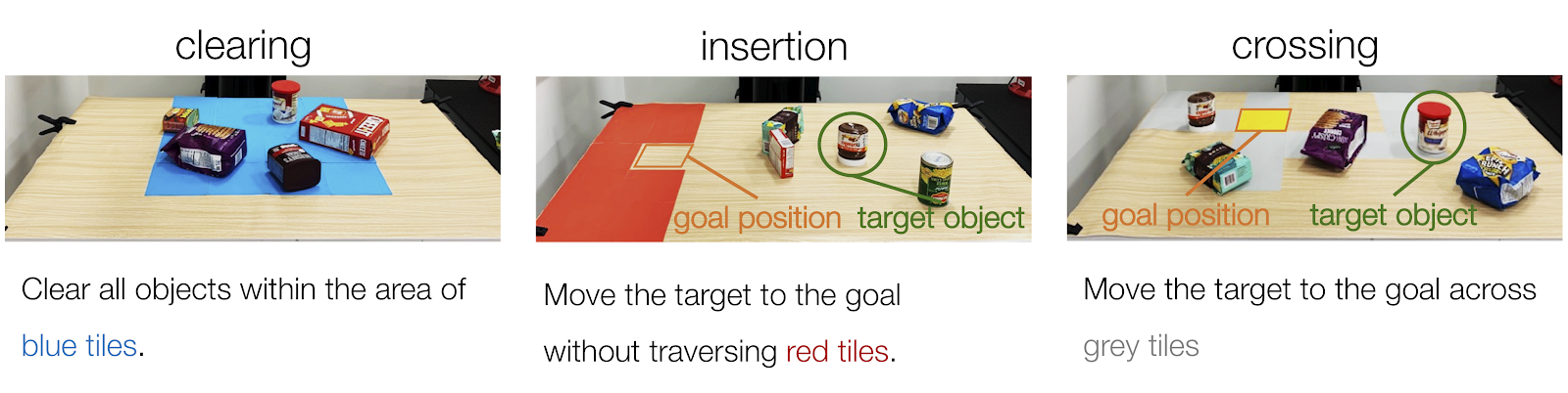
Open Path: When the target object is surrounded by obstacle objects, the robot opens a path for the target object (the red canned meat) towards the goal without entering the restricted area (red tiles).
Get Around: In the presence of a pile of obstacle objects between the target (the blue bag of snacks) and the goal, the robot pushes the target around.
Squeeze Through: When there is a small gap between a bunch of objects, the robot squeezes the target object (the blue tuna can) through the gap.
Move Away Obstacles: When pushing the target object (the red jello box) across the bridge (grey tiles), the robot clears obstacle objects one by one along the way.
Push Target Through Obstacles: When the robot cannot directly reach the target object (tuna can), it squeezes the target object by pushing obstacle objects.
Clean up a workspace: The robot moves objects out of a designated workspace (blue tiles).
Summary
We proposed CAVIN, a hierarchical planning algorithm in learned latent spaces. Using deep generative models, CAVIN prioritizes useful actions in sampling-based planning. The planning process is factored into two levels by subgoals to effectively generate plans. A cascaded variational inference framework is used to learn CAVIN from task-agnostic interactions. Our method enables the robot to effectively perform multi-step manipulation tasks in cluttered tabletop environments given high-dimensional visual inputs.
We expect to apply CAVIN in more challenging multi-step manipulation tasks in the future. While the core algorithm is not limited to the planar pushing actions demonstrated in this work, how to effectively solve sequential problems which require diverse robot skills such as grasping, sweeping, hammering, etc. still remains an open question. While in our tasks we assume all objects are placed on the table without occlusions, the robot will need to explicitly deal with partial observations in more complex environments.
For more information please refer to the project website. We’ve also released our codebase and the robotic task environments in simulation and the real world.
This blog post was based on the following paper: Dynamics Learning with Cascaded Variational Inference for Multi-Step Manipulation. K. Fang, Y. Zhu, A. Garg, S.Savarese, L. Fei-Fei. In Conference on Robot Learning, 2019. (pdf)
Reducing delays in wireless networks
MIT researchers have designed a congestion-control scheme for wireless networks that could help reduce lag times and increase quality in video streaming, video chat, mobile gaming, and other web services.
To keep web services running smoothly, congestion-control schemes infer information about a network’s bandwidth capacity and congestion based on feedback from the network routers, which is encoded in data packets. That information determines how fast data packets are sent through the network.
Deciding a good sending rate can be a tough balancing act. Senders don’t want to be overly conservative: If a network’s capacity constantly varies from, say, 2 megabytes per second to 500 kilobytes per second, the sender could always send traffic at the lowest rate. But then your Netflix video, for example, will be unnecessarily low-quality. On the other hand, if the sender constantly maintains a high rate, even when network capacity dips, it could overwhelm the network, creating a massive queue of data packets waiting to be delivered. Queued packets can increase the network’s delay, causing, say, your Skype call to freeze.
Things get even more complicated in wireless networks, which have “time-varying links,” with rapid, unpredictable capacity shifts. Depending on various factors, such as the number of network users, cell tower locations, and even surrounding buildings, capacities can double or drop to zero within fractions of a second. In a paper at the USENIX Symposium on Networked Systems Design and Implementation, the researchers presented “Accel-Brake Control” (ABC), a simple scheme that achieves about 50 percent higher throughput, and about half the network delays, on time-varying links.
The scheme relies on a novel algorithm that enables the routers to explicitly communicate how many data packets should flow through a network to avoid congestion but fully utilize the network. It provides that detailed information from bottlenecks — such as packets queued between cell towers and senders — by repurposing a single bit already available in internet packets. The researchers are already in talks with mobile network operators to test the scheme.
“In cellular networks, your fraction of data capacity changes rapidly, causing lags in your service. Traditional schemes are too slow to adapt to those shifts,” says first author Prateesh Goyal, a graduate student in CSAIL. “ABC provides detailed feedback about those shifts, whether it’s gone up or down, using a single data bit.”
Joining Goyal on the paper are Anup Agarwal, now a graduate student at Carnegie Melon University; Ravi Netravali, now an assistant professor of computer science at the University of California at Los Angeles; Mohammad Alizadeh, an associate professor in MIT’s Department of Electrical Engineering (EECS) and CSAIL; and Hari Balakrishnan, the Fujitsu Professor in EECS. The authors have all been members of the Networks and Mobile Systems group at CSAIL.
Achieving explicit control
Traditional congestion-control schemes rely on either packet losses or information from a single “congestion” bit in internet packets to infer congestion and slow down. A router, such as a base station, will mark the bit to alert a sender — say, a video server — that its sent data packets are in a long queue, signaling congestion. In response, the sender will then reduce its rate by sending fewer packets. The sender also reduces its rate if it detects a pattern of packets being dropped before reaching the receiver.
In attempts to provide greater information about bottlenecked links on a network path, researchers have proposed “explicit” schemes that include multiple bits in packets that specify current rates. But this approach would mean completely changing the way the internet sends data, and it has proved impossible to deploy.
“It’s a tall task,” Alizadeh says. “You’d have to make invasive changes to the standard Internet Protocol (IP) for sending data packets. You’d have to convince all Internet parties, mobile network operators, ISPs, and cell towers to change the way they send and receive data packets. That’s not going to happen.”
With ABC, the researchers still use the available single bit in each data packet, but they do so in such a way that the bits, aggregated across multiple data packets, can provide the needed real-time rate information to senders. The scheme tracks each data packet in a round-trip loop, from sender to base station to receiver. The base station marks the bit in each packet with “accelerate” or “brake,” based on the current network bandwidth. When the packet is received, the marked bit tells the sender to increase or decrease the “in-flight” packets — packets sent but not received — that can be in the network.
If it receives an accelerate command, it means the packet made good time and the network has spare capacity. The sender then sends two packets: one to replace the packet that was received and another to utilize the spare capacity. When told to brake, the sender decreases its in-flight packets by one — meaning it doesn’t replace the packet that was received.
Used across all packets in the network, that one bit of information becomes a powerful feedback tool that tells senders their sending rates with high precision. Within a couple hundred milliseconds, it can vary a sender’s rate between zero and double. “You’d think one bit wouldn’t carry enough information,” Alizadeh says. “But, by aggregating single-bit feedback across a stream of packets, we can get the same effect as that of a multibit signal.”
Staying one step ahead
At the core of ABC is an algorithm that predicts the aggregate rate of the senders one round-trip ahead to better compute the accelerate/brake feedback.
The idea is that an ABC-equipped base station knows how senders will behave — maintaining, increasing, or decreasing their in-flight packets — based on how it marked the packet it sent to a receiver. The moment the base station sends a packet, it knows how many packets it will receive from the sender in exactly one round-trip’s time in the future. It uses that information to mark the packets to more accurately match the sender’s rate to the current network capacity.
In simulations of cellular networks, compared to traditional congestion control schemes, ABC achieves around 30 to 40 percent greater throughput for roughly the same delays. Alternatively, it can reduce delays by around 200 to 400 percent by maintaining the same throughput as traditional schemes. Compared to existing explicit schemes that were not designed for time-varying links, ABC reduces delays by half for the same throughput. “Basically, existing schemes get low throughput and low delays, or high throughput and high delays, whereas ABC achieves high throughput with low delays,” Goyal says.
Next, the researchers are trying to see if apps and web services can use ABC to better control the quality of content. For example, “a video content provider could use ABC’s information about congestion and data rates to pick the resolution of streaming video more intelligently,” Alizadeh says. “If it doesn’t have enough capacity, the video server could lower the resolution temporarily, so the video will continue playing at the highest possible quality without freezing.”

How Airbus Detects Anomalies in ISS Telemetry Data Using TFX
A guest post by Philipp Grashorn, Jonas Hansen and Marcel Rummens from Airbus
 |
| The International Space Station and it’s different modules. Airbus designed and built the Columbus module in 2008. |
Airbus provides several services for the operation of the Columbus module and its payloads on the International Space Station (ISS). Columbus was launched in 2008 and is one of the main laboratories onboard the ISS. To ensure the health of the crew as well as hundreds of systems onboard the Columbus module, engineers have to keep track of many telemetry datastreams, which are constantly beamed to earth.
The operations team at the Columbus Control Center, in collaboration with Airbus, keeps track of thousands of parameters, monitored in 24/7 shifts. If an operator detects an anomaly, he or she creates an anomaly report which is resolved by Airbus system experts. The team at Airbus created the ISS Analytics project to automate part of the workflow of detecting anomalies.
 |
| Previous, manual workflow |
Detecting Anomalies
The Columbus module consists of several subsystems, each of which is composed of multiple components, resulting in about 17,000 unique telemetry parameters. As each subsystem is highly specialized, it made sense to train a separate model for each subsystem.
Lambda Architecture
In order to detect anomalies within the real time telemetry data stream, the models are trained on about 10 years worth of historical data, which is constantly streamed to earth and stored in a specialized database. On average, the data is streamed in a frequency of one hertz. Simply looking at the data of the last 10 years results in over 5 trillion data points, (10y * 365d * 24h * 60min * 60s * 17K params).
A problem of this magnitude requires big data technologies and a level of computational power which is typically only found in the cloud. As of now a public cloud was adopted, however as more sensitive systems are integrated in the future, the project has to be migrated to the Airbus Private Cloud for security purposes.
To tackle this anomaly detection problem, a lambda architecture was designed which is composed of two parts: the speed and the batch layer.
 |
| High Level architecture of ISS Analytics |
The batch layer consists only of the learning pipeline, fed with historical time series data which is queried from an on-premise database. Using an on-premise Spark cluster, the data is sanitized and prepared for the upload to GCP. TFX on Kubeflow is used to train an LSTM Autoencoder (details in the next section) and deploy it using TF-Serving.
The speed layer is responsible for monitoring the real-time telemetry stream, which is received using multiple ground stations on earth. The monitoring process uses the deployed TensorFlow model to detect anomalies and compare them against a database of previously detected anomalies, simplifying the root cause analysis and decreasing the time to resolution. In case the neural network detects an anomaly, a reporting service is triggered which consolidates all important information related to the potential anomaly. A notification service then creates an abstract and informs the responsible experts.
Training an Autoencoder to Detect Anomalies
As mentioned above, each model is trained on a subset of telemetry parameters. The objective of the model is to represent the nominal state of the subsystem. If the model is able to reconstruct observations of nominal states with a high accuracy, it will have difficulties reconstructing observations of states which deviate from the nominal state. Thus, the reconstruction error of the model is used as an indicator for anomalies during inference, as well as part of the cost function in training. Details of this practice can be found here and here.
The anomaly detection approach outlined above was implemented using a special type of artificial neural network called an Autoencoder. An Autoencoder can be divided into two parts: the encoder and the decoder. The encoder is a mapping from the input space into a lower dimensional latent space. The decoder is a mapping from the latent space into the reconstruction space with a dimensionality equal to the input space.
While the encoder generates a compressed representation of the input, the decoder generates a representation as close as possible to the original input, using the latent vector from the encoder. Dimensionality reduction acts as a funnel which enables the autoencoder to ignore signal noise.
The difference between the input and the reconstruction is called reconstruction error and is calculated as the root-mean-square error. The reconstruction error, as mentioned above, is minimized in the training step and acts as an indicator for anomalies during inference (e.g., an anomaly would have high reconstruction error).
 |
| Example Architecture of an Autoencoder |
LSTM for sequences
The Autoencoder uses LSTMs to process sequences and capture temporal information. Each observation is represented as a tensor with shape [number_of_features,number_of_timesteps_per_sequence]. The data is prepared using TFT’s scale_to_0_1 and vocabulary functions. Each LSTM layer of the encoder is followed by an instance of tf.keras.layers.Dropout to increase the robustness against noise.
 |
| Model Architecture of ISS Analytics (Red circles represent dropout) |
Using TFX
The developed solution contains many but not all of the TensorFlow Extended (TFX) components. However it is planned to research and integrate additional components included with the TFX suite in the future.
The library that is most used in this solution is tf.Transform, which processes the raw telemetry data and converts it into a format compatible with the Autoencoder model. The preprocessing steps are defined in the preprocessing_fn() function and executed on Apache Beam. The resulting transformation graph is stored hermetically within the graph of the trained model. This ensures that the raw data is always processed using the same function, independent of the environment it is deployed in. This way the data fed into the model is consistent.
The sequence-based approach which was outlined in an earlier section posed some challenges. The input_fn() of model training reads the data, preprocessed in the preceding tf.Transform step and applies a windowing function to create sequences. This step is necessary because the data is stored as time steps without any sequence information. Afterwards, it creates batches of size sequence_length * batch_size and converts the whole dataset into a sparse tensor for the input layer of the Autoencoder (tf.contrib.feature_column.sequence_input_layer()expects sparse tensors).
The serving_input_fn() on the other hand receives already sequenced data from upstream systems (data-stream from the ISS). But this data is not yet preprocessed and therefore the tf.Transform step has to be applied. This step is preceded and followed by reshaping calls, in order to temporarily remove the sequence-dimension of the tensor for the preprocessing_fn().
Orchestration for all parts of the machine learning pipeline (transform, train, evaluate) was done with Kubeflow Pipelines. This toolkit simplifies and accelerates the process of training models, experimenting with different architectures and optimizing hyperparameters. By leveraging the benefits of Kubernetes on GCP, it is very convenient to run multiple experiments in parallel. In combination with the Kubeflow UI, one can analyze the hyperparameters and results of these runs in a well-structured form. For a more detailed analysis of specific models and runs, TensorBoard was used to examine learning curves and neural network topologies.
The last step in this TFX use case is to connect the batch and the speed layer by deploying the trained model with TensorFlow Serving. This turned out to be the most important component of TFX, actually bringing the whole machine learning system into production. Its support for features like basic monitoring, a standardized API, effortless rollover and A/B testing, have been crucial for this project.
With the modular design of TFX pipelines, it was possible to train separate models for many subsystems of the Columbus module, without any major modifications. Serving these models as independent services on Kubernetes allows scaling the solution, in order to apply anomaly detection to multiple subsystems in parallel.
Utilizing TFX on Kubeflow brought many benefits to the project. Its flexible nature allows a seamless transition between different environments and will help the upcoming migration to the Airbus Private Cloud. In addition, the work done by this project can be repurposed to other products without any major rework, utilizing the development of generic and reusable TFX components.
Combining all these features the system is now capable of analysing large amounts of telemetry parameters, detecting anomalies and triggering the required steps for a faster and smarter resolution.
 |
| The partially automated workflow after the ISS Analytics project |
To learn more about Airbus checkout out the Airbus website or dive deeper into the Airbus Space Infrastructure. To learn more about TFX check out the TFX website, join the TFX discussion group, dive into other posts in the TFX blog, or watch the TFX playlist on YouTube.
Learning computational tasks from single examples
New “meta-learning” approach improves on the state of the art in “one-shot” learning.Read More
Bluetooth signals from your smartphone could automate Covid-19 contact tracing while preserving privacy
Imagine you’ve been diagnosed as Covid-19 positive. Health officials begin contact tracing to contain infections, asking you to identify people with whom you’ve been in close contact. The obvious people come to mind — your family, your coworkers. But what about the woman ahead of you in line last week at the pharmacy, or the man bagging your groceries? Or any of the other strangers you may have come close to in the past 14 days?
A team led by MIT researchers and including experts from many institutions is developing a system that augments “manual” contact tracing by public health officials, while preserving the privacy of all individuals. The system relies on short-range Bluetooth signals emitted from people’s smartphones. These signals represent random strings of numbers, likened to “chirps” that other nearby smartphones can remember hearing.
If a person tests positive, they can upload the list of chirps their phone has put out in the past 14 days to a database. Other people can then scan the database to see if any of those chirps match the ones picked up by their phones. If there’s a match, a notification will inform that person that they may have been exposed to the virus, and will include information from public health authorities on next steps to take. Vitally, this entire process is done while maintaining the privacy of those who are Covid-19 positive and those wishing to check if they have been in contact with an infected person.
“I keep track of what I’ve broadcasted, and you keep track of what you’ve heard, and this will allow us to tell if someone was in close proximity to an infected person,” says Ron Rivest, MIT Institute Professor and principal investigator of the project. “But for these broadcasts, we’re using cryptographic techniques to generate random, rotating numbers that are not just anonymous, but pseudonymous, constantly changing their ‘ID,’ and that can’t be traced back to an individual.”
This approach to private, automated contact tracing will be available in a number of ways, including through the privacy-first effort launched at MIT in response to Covid-19 called SafePaths. This broad set of mobile apps is under development by a team led by Ramesh Raskar of the MIT Media Lab. The design of the new Bluetooth-based system has benefited from SafePaths’ early work in this area.
Bluetooth exchanges
Smartphones already have the ability to advertise their presence to other devices via Bluetooth. Apple’s “Find My” feature, for example, uses chirps from a lost iPhone or MacBook to catch the attention of other Apple devices, helping the owner of the lost device to eventually find it.
“Find My inspired this system. If my phone is lost, it can start broadcasting a Bluetooth signal that’s just a random number; it’s like being in the middle of the ocean and waving a light. If someone walks by with Bluetooth enabled, their phone doesn’t know anything about me; it will just tell Apple, ‘Hey, I saw this light,’” says Marc Zissman, the associate head of MIT Lincoln Laboratory’s Cyber Security and Information Science Division and co-principal investigator of the project.
With their system, the team is essentially asking a phone to send out this kind of random signal all the time and to keep a log of these signals. At the same time, the phone detects chirps it has picked up from other phones, and only logs chirps that would be medically significant for contact tracing — those emitted from within an approximate 6-foot radius and picked up for a certain duration of time, say 10 minutes.
Phone owners would get involved by downloading an app that enables this system. After a positive diagnosis, a person would receive a QR code from a health official. By scanning the code through that app, that person can upload their log to the cloud. Anyone with the app could then initiate their phones to scan these logs. A notification, if there’s a match, could tell a user how long they were near an infected person and the approximate distance.
Privacy-preserving technology
Some countries most successful at containing the spread of Covid-19 have been using smartphone-based approaches to conduct contact tracing, yet the researchers note these approaches have not always protected individual’s privacy. South Korea, for example, has implemented apps that notify officials if a diagnosed person has left their home, and can tap into people’s GPS data to pinpoint exactly where they’ve been.
“We’re not tracking location, not using GPS, not attaching your personal ID or phone number to any of these random numbers your phone is emitting,” says Daniel Weitzner, a principal research scientist in the MIT Computer Science and Artificial Intelligence Laboratory (CSAIL) and co-principal investigator of this effort. “What we want is to enable everyone to participate in a shared process of seeing if you might have been in contact, without revealing, or forcing anyone to reveal, anything.”
Choice is key. Weitzner sees the system as a virtual knock on the door that preserves people’s right to not answer it. The hope, though, is that everyone who can opt in would do so to help contain the spread of Covid-19. “We need a large percentage of the population to opt in for this system to really work. We care about every single Bluetooth device out there; it’s really critical to make this a whole ecosystem,” he says.
Public health impact
Throughout the development process, the researchers have worked closely with a medical advisory team to ensure that this system would contribute effectively to contact tracing efforts. This team is led by Louise Ivers, who is an infectious disease expert, associate professor at Harvard Medical School, and executive director of the Massachusetts General Hospital Center for Global Health.
“In order for the U.S. to really contain this epidemic, we need to have a much more proactive approach that allows us to trace more widely contacts for confirmed cases. This automated and privacy-protecting approach could really transform our ability to get the epidemic under control here and could be adapted to have use in other global settings,” Ivers says. “What’s also great is that the technology can be flexible to how public health officials want to manage contacts with exposed cases in their specific region, which may change over time.”
For example, the system could notify someone that they should self-isolate, or it could request that they check in through the app to connect with specialists regarding daily symptoms and well-being. In other circumstances, public health officials could request that this person get tested if they were noticing a cluster of cases.
The ability to conduct contact tracing quickly and at a large scale can be effective not only in flattening the curve of the outbreak, but also for enabling people to safely enter public life once a community is on the downward side of the curve. “We want to be able to let people carefully get back to normal life while also having this ability to carefully quarantine and identify certain vectors of an outbreak,” Rivest says.
Toward implementation
Lincoln Laboratory engineers have led the prototyping of the system. One of the hardest technical challenges has been achieving interoperability, that is, making it possible for a chirp from an iPhone to be picked up by an Android device and vice versa. A test at the laboratory late last week proved that they achieved this capability, and that chirps could be picked up by other phones of various makes and models.
A vital next step toward implementation is engaging with the smartphone manufacturers and software developers — Apple, Google, and Microsoft. “They have a critical role here. The aim of the prototype is to prove to these developers that this is feasible for them to implement,” Rivest says. As those collaborations are forming, the team is also demonstrating its prototype system to state and federal government agencies.
Rivest emphasizes that collaboration has made this project possible. These collaborators include the Massachusetts General Hospital Center for Global Health, CSAIL, MIT Lincoln Laboratory, Boston University, Brown University, MIT Media Lab, The Weizmann Institute of Science, and SRI International.
The team also aims to play a central, coordinating role with other efforts around the country and in Europe to develop similar, privacy-preserving contact-tracing systems.
“This project is being done in true academic style. It’s not a contest; it’s a collective effort on the part of many, many people to get a system working,” Rivest says.
Amazon German R&D center is dedicated to open AI research
‘Lablet’s’ leader, Yasser Jadidi, says the research center’s mission aligns with Amazon’s customer orientation and its responsibility to society.Read More
Sprayable user interfaces
For decades researchers have envisioned a world where digital user interfaces are seamlessly integrated with the physical environment, until the two are virtually indistinguishable from one another.
This vision, though, is held up by a few boundaries. First, it’s difficult to integrate sensors and display elements into our tangible world due to various design constraints. Second, most methods to do so are limited to smaller scales, bound by the size of the fabricating device.
Recently, a group of researchers from MIT’s Computer Science and Artificial Intelligence Laboratory (CSAIL) came up with SprayableTech, a system that lets users create room-sized interactive surfaces with sensors and displays. The system, which uses airbrushing of functional inks, enables various displays, like interactive sofas with embedded sensors to control your television, and sensors for adjusting lighting and temperature through your walls.
SprayableTech lets users channel their inner Picassos: After designing your interactive artwork in the 3D editor, it automatically generates stencils for airbrushing the layout onto a surface. Once they’ve created the stencils from cardboard, a user can then add sensors to the desired surface, whether it’s a sofa, a wall, or even a building, to control various appliances like your lamp or television. (An alternate option to stenciling is projecting them digitally.)
“Since SprayableTech is so flexible in its application, you can imagine using this type of system beyond walls and surfaces to power larger-scale entities like interactive smart cities and interactive architecture in public places,” says Michael Wessely, postdoc in CSAIL and lead author on a new paper about SprayableTech. “We view this as a tool that will allow humans to interact with and use their environment in newfound ways.”
The race for the smartest home has now been in the works for some time, with a large interest in sensor technology. It’s a big advance from the enormous glass wall displays with quick-shifting images and screens we’ve seen in countless dystopian films.
The MIT researchers’ approach is focusing on scale, and creative expression. By using the airbrush technology, they’re no longer limited to the size of the printer, the area of the screen-printing net, or the size of the hydrographic bath — and there’s thousands of possible design options.
Let’s say a user wanted to design a tree symbol on their wall to control the ambient light in the room. To start the process, they would use a toolkit in a 3D editor to design their digital object, and customize for things like proximity sensors, touch buttons, sliders, and electroluminescent displays.
Then, the toolkit would output the choice of stencils: fabricated stencils cut from cardboard, which are great for high-precision spraying on simple, flat, surfaces, or projected stencils, which are less precise, but better for doubly-curved surfaces.
Designers can then spray on the functional ink, which is ink with electrically functional elements, using an airbrush. As a final step to get the system going, a microcontroller is attached that connects the interface to the board that runs the code for sensing and visual output.
The team tested the system on a variety of items, including:
- a musical interface on a concrete pillar;
- an interactive sofa that’s connected to a television;
- a wall display for controlling light; and
- a street post with a touchable display that provides audible information on subway stations and local attractions.
Since the stencils need to be created in advance via the digital editor, it reduces the opportunity for spontaneous exploration. Looking forward, the team wants to explore so-called “modular” stencils that create touch buttons of different sizes, as well as shape-changing stencils that adjust themselves based on a desired user interface shape.
“In the future, we aim to collaborate with graffiti artists and architects to explore the future potential for large-scale user interfaces in enabling the internet of things for smart cities and interactive homes,” says Wessely.
Wessely wrote the paper alongside MIT PhD student Ticha Sethapakdi, MIT undergraduate students Carlos Castillo and Jackson C. Snowden, MIT postdoc Isabel P.S. Qamar, MIT Professor Stefanie Mueller, University of Bristol PhD student Ollie Hanton, University of Bristol Professor Mike Fraser, and University of Bristol Associate Professor Anne Roudaut.