Aerobotics improves training speed by 24 times per sample with Amazon SageMaker and TensorFlow

Editor’s note: This is a guest post written by Michael Malahe, Head of Data at Aerobotics, a South African startup that builds AI-driven tools for agriculture.

Aerobotics is an agri-tech company operating in 18 countries around the world, based out of Cape Town, South Africa. Our mission is to provide intelligent tools to feed the world. We aim to achieve this by providing farmers with actionable data and insights on our platform, Aeroview, so that they can make the necessary interventions at the right time in the growing season. Our predominant data source is aerial drone imagery: capturing visual and multispectral images of trees and fruit in an orchard.

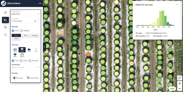
In this post we look at how we use Amazon SageMaker and TensorFlow to improve our Tree Insights product, which provides per-tree measurements of important quantities like canopy area and health, and provides the locations of dead and missing trees. Farmers use this information to make precise interventions like fixing irrigation lines, applying fertilizers at variable rates, and ordering replacement trees. The following is an image of the tool that farmers use to understand the health of their trees and make some of these decisions.

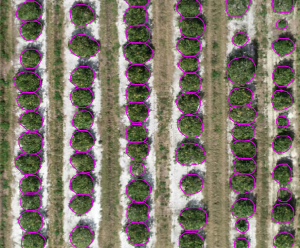
To provide this information to make these decisions, we first must accurately assign each foreground pixel to a single unique tree. For this instance segmentation task, it’s important that we’re as accurate as possible, so we use a machine learning (ML) model that’s been effective in large-scale benchmarks. The model is a variant of Mask R-CNN, which pairs a convolutional neural network (CNN) for feature extraction with several additional components for detection, classification, and segmentation. In the following image, we show some typical outputs, where the pixels belong to a given tree are outlined by a contour.

Glancing at the outputs, you might think that the problem is solved.

The challenge

The main challenge with analyzing and modeling agricultural data is that it’s highly varied across a number of dimensions.

The following image illustrates some extremes of the variation in the size of trees and the extent to which they can be unambiguously separated.

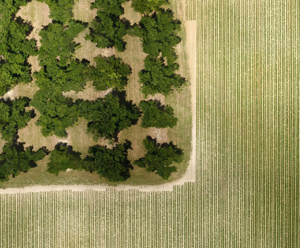
In the grove of pecan trees, we have one of the largest trees in our database, with an area of 654 m2 (a little over a minute to walk around at a typical speed). The vines to the right of the grove measure 50 cm across (the size of a typical potted plant). Our models need to be tolerant to these variations to provide accurate segmentations regardless of the scale.

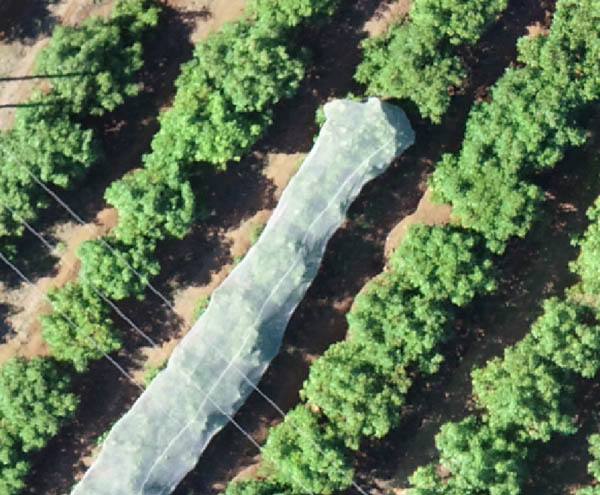
An additional challenge is that the sources of variation aren’t static. Farmers are highly innovative, and best practices can change significantly over time. One example is ultra-high-density planting for apples, where trees are planted as close as a foot apart. Another is the adoption of protective netting, which obscures aerial imagery, as in the following image.

In this domain with broad and shifting variations, we need to maintain accurate models to provide our clients with reliable insights. Models should improve with every challenging new sample we encounter, and we should deploy them with confidence.

In our initial approach to this challenge, we simply trained on all the data we had. As we scaled, however, we quickly got to the point where training on all our data became infeasible, and the cost of doing so became an impediment to experimentation.

The solution

Although we have variation in the edge cases, we recognized that there was a lot of redundancy in our standard cases. Our goal was to get to a point where our models are trained on only the most salient data, and can converge without needing to see every sample. Our approach to achieving this was first to create an environment where it’s simple to experiment with different approaches to dataset construction and sampling. The following diagram shows our overall workflow for the data preprocessing that enables this.

The outcome is that training samples are available as individual files in Amazon Simple Storage Service (Amazon S3), which is only sensible to do with bulky data like multispectral imagery, with references and rich metadata stored in Amazon Redshift tables. This makes it trivial to construct datasets with a single query, and makes it possible to fetch individual samples with arbitrary access patterns at train time. We use UNLOAD to create an immutable dataset in Amazon S3, and we create a reference to the file in our Amazon Relational Database Service (Amazon RDS) database, which we use for training provenance and evaluation result tracking. See the following code:

UNLOAD ('[subset_query]')
TO '[s3://path/to/dataset]'
IAM_ROLE '[redshift_write_to_s3_role]'
FORMAT PARQUET

The ease of querying the tile metadata allowed us to rapidly create and test subsets of our data, and eventually we were able to train to convergence after seeing only 1.1 million samples of a total 3.1 million. This sub-epoch convergence has been very beneficial in bringing down our compute costs, and we got a better understanding of our data along the way.

The second step we took in reducing our training costs was to optimize our compute. We used the TensorFlow profiler heavily throughout this step:

import tensorflow as tf
tf.profiler.experimental.ProfilerOptions(host_tracer_level=2,  python_tracer_level=1,device_tracer_level=1)
tf.profiler.experimental.start("[log_dir]")
[train model]
tf.profiler.experimental.stop()

For training, we use Amazon SageMaker with P3 instances provisioned by Amazon Elastic Compute Cloud (Amazon EC2), and initially we found that the NVIDIA Tesla V100 GPUs in the instances were bottlenecked by CPU compute in the input pipeline. The overall pattern for alleviating the bottleneck was to shift as much of the compute from native Python code to TensorFlow operations as possible to ensure efficient thread parallelism. The largest benefit was switching to tf.io for data fetching and deserialization, which improved throughput by 41%. See the following code:

serialised_example = tf.io.decode_compressed(tf.io.gfile.GFile(fname, 'rb').read(), compression_type='GZIP')
example = tf.train.Example.FromString(serialised_example.numpy())

A bonus feature with this approach was that switching between local files and Amazon S3 storage required no code changes due to the file object abstraction provided by GFile.

We found that the last remaining bottleneck came from the default TensorFlow CPU parallelism settings, which we optimized using a SageMaker hyperparameter tuning job (see the following example config).

With the CPU bottleneck removed, we moved to GPU optimization, and made the most of the V100’s Tensor Cores by using mixed precision training:

from tensorflow.keras.mixed_precision import experimental as mixed_precision
policy = mixed_precision.Policy('mixed_float16')
mixed_precision.set_policy(policy)

The mixed precision guide is a solid reference, but the change to using mixed precision still requires some close attention to ensure that the operations happening in half precision are not ill-conditioned or prone to underflow. Some specific cases that were critical were terminal activations and custom regularization terms. See the following code:

import tensorflow as tf
...
y_pred = tf.keras.layers.Activation('sigmoid', dtype=tf.float32)(x)
loss = binary_crossentropy(tf.cast(y_true, tf.float32), tf.cast(y_pred, tf.float32), from_logits=True)
...
model.add_loss(lambda: tf.keras.regularizers.l2()(tf.cast(w, tf.float32)))

After implementing this, we measured the following benchmark results for a single V100.

Precision CPU parallelism Batch size Samples per second
single default 8 9.8
mixed default 16 19.3
mixed optimized 16 22.4

The impact of switching to mixed precision was that training speed roughly doubled, and the impact of using the optimal CPU parallelism settings discovered by SageMaker was an additional 16% increase.

Implementing these initiatives as we grew resulted in reducing the cost of training a model from $122 to $68, while our dataset grew from 228 thousand samples to 3.1 million, amounting to a 24 times reduction in cost per sample.

Conclusion

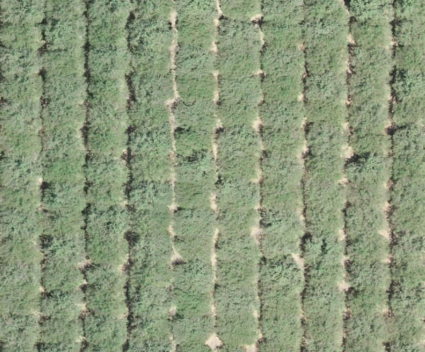
This reduction in training time and cost has meant that we can quickly and cheaply adapt to changes in our data distribution. We often encounter new cases that are confounding even for humans, such as the following image.

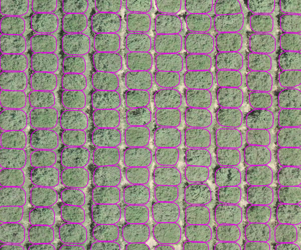
However, they quickly become standard cases for our models, as shown in the following image.

We aim to continue making training faster by using more devices, and making it more efficient by leveraging SageMaker managed Spot Instances. We also aim to make the training loop tighter by serving SageMaker models that are capable of online learning, so that improved models are available in near-real time. With these in place, we should be well equipped to handle all the variation that agriculture can throw at us. To learn more about Amazon SageMaker, visit the product page.


The content and opinions in this post are those of the third-party author and AWS is not responsible for the content or accuracy of this post.


About the Author

Michael Malahe is the Head of Data at Aerobotics, a South African startup that builds AI-driven tools for agriculture.

Read More

Shackling Jitter and Perfecting Ping, How to Reduce Latency in Cloud Gaming

Looking to improve your cloud gaming experience? First, become a master of your network.

Twitch-class champions in cloud gaming shred Wi-Fi and broadband waves. They cultivate good ping to defeat two enemies — latency and jitter.

What Is Latency? 

Latency or lag is a delay in getting data from the device in your hands to a computer in the cloud and back again.

What Is Jitter?

Jitter is the annoying disruption you feel that leads to yelling at your router, (“You’re breaking up, again!”) when pieces of that data (called packets) get sidetracked.

Why Are Latency and Jitter Important?

Cloud gaming works by rendering game images on a custom GFN server that may be miles away, those images are then sent to a game server, and finally appear on the device in front of you.

When you fire at an enemy, your device sends data packets to these servers. The kill happens on the game on those servers, sending back commands that display the win on your screen.

And it all happens in less than the blink of an eye. In technical terms, it’s measured in “ping.”

What Is Ping?

Ping in is the time in milliseconds it takes a data packet to go to the server and back.

Anyone with the right tools and a little research can prune their ping down to less than 30 milliseconds. Novices can get pummeled with as much as 300 milliseconds of lag. It’s the difference between getting or being the game-winning kill.

Before we describe the ways to crush latency and jitter, let’s take its measure.

To Measure Latency, Test Your Ping

Speedtest.net and speedsmart.net are easy to take, but they only measure the latency to a generic server that may be in your network.

It doesn’t measure the time it takes to get data to and from the server you’re connecting to for your cloud gaming session. For a more accurate gauge of your ping, some cloud gaming services, such as NVIDIA GeForce NOW, sport their own built-in test for network latency. Those network tests will measure the ping time to and the respective cloud gaming server.

Blazing Wi-Fi and broadband can give your ping some zing.

My Speedtest result showed a blazing 10 milliseconds, while Speedsmart measured a respectable 23ms.

Your mileage may vary, too. If it sticks its head much up over 30ms, the first thing to do is check your ISP or network connection. Still having trouble? Try rebooting. Turn your device and your Wi-Fi network off for 10 seconds, then turn them back on and run the tests again.

How to Reduce Latency and Ping

If the lag remains, more can be done for little or no cost, and new capabilities are coming down the pike that will make things even better.

First, try to get off Wi-Fi. Simply running a standard Ethernet cable from your Wi-Fi router to your device can slash latency big time.

If you can’t do that, there are still plenty of ways to tune your Wi-Fi.

Ethernet is faster, but research from CableLabs shows most gamers use Wi-Fi.

Your ping may be stuck in heavy traffic. Turn off anything else running on your Wi-Fi network, especially streaming videos, work VPNs — hey, it’s time for play — and anyone trying to download the Smithsonian archives.

A High Five Can Avoid Interference

If rush-hour traffic is unavoidable on your home network, you can still create your own diamond lane.

Unless you have an ancient Wi-Fi access point (AP, for short — often referred to as a router) suitable for display in a museum, it should support both 2.4- and 5GHz channels.

You can claw back many milliseconds of latency if you shunt most of your devices to the 2.4GHz band and save 5GHz for cloud gaming.

Apps called Wi-Fi analyzers on the Android and iTunes stores can even determine which slices of your Wi-Fi airspace are more or less crowded. A nice fat 80MHz channel in the 5GHz band without much going on nearby is an ideal runway for cloud gaming.

Quash Latency with QoS

If it’s less than a decade old, your AP probably has something called quality of service, or QoS.

QoS can give some apps higher priority than others. APs vary widely in how they implement QoS, but it’s worth checking to see if your network can be set to give priority to cloud gaming.

NVIDIA provides a list of the recommended AP it’s tested with GeForce NOW as well as a support page for how to apply QoS and other techniques.

Take a Position Against Latency

If latency persists, see if you can get physically closer to your AP. Can you move to the same room?

If not, consider buying a mesh network. That’s a collection of APs you can string around your home, typically with Ethernet cables, so you have an AP in every room where you use Wi-Fi.

Some folks suggest trying different positions for your router and your device to get the sweetest reception. But others say this will only shave a millisecond or so off your lag at best, so don’t waste too much time playing Wi-Fi yoga.

Stay Tuned for Better Ping

The good news is more help is on the way. The latest version, Wi-Fi 6, borrows a connection technology from cellular networks (called OFDMA) that reduces signal interference significantly, reducing latency.

So, if you can afford it, get a Wi-Fi 6 AP, but you’ll have to buy a gaming device that supports Wi-Fi 6, too.

Next year, Wi-Fi 6E devices should be available. They’ll sport a new 6MHz Wi-Fi band where you can find fresh channels for gaming.

Coping with Internet Latency

Your broadband connection is the other part of the net you need to set up for cloud gaming. First, make sure your internet plan matches the kind of cloud gaming you want to play.

These days a basic plan tops out at about 15 Mbits/second. That’s enough if your screen can display 1280×720 pixels, aka standard high definition or 720p. If you want a smoother, more responsive experience, step up to 1080p resolution, full high def or even 4K ultra-high def — this requires at least 25 Mbits/s. More is always better.

If you’re playing on a smartphone, 5G cellular services are typically the fastest links, but in some areas a 4G LTE service may be well optimized for gaming. It’s worth checking the options with your cellular provider.

When logging into your cloud gaming service, choosing the closest server can make a world of difference.

For example, using the speedsmart.net test gave me a ping of 29ms from a server in San Francisco, 41 miles away. Choosing a server in Atlanta, more than 2,000 miles away, bloated my ping to 80ms. And forget about even trying to play on a server on another continent.

GeForce NOW members can sit back and relax on this one. The service automatically picks the fastest server for you, even if the server is a bit farther away.

A Broadband Horizon for Cloud Gaming

Internet providers want to tame the latency and jitter in their broadband networks, too.

Cable operators plan to upgrade their software, called DOCSIS 3.1, to create low-latency paths for cloud gamers. A version of the software, called L4S, for other kinds of internet access providers and Wi-Fi APs is also in the works.

Broadband latency should shrink to a fraction of its size (from blue to red in the chart) once low-latency DOCSIS 3.1 software is available and supported.

The approach requires some work on the part of application developers and cloud gaming services. But the good news is engineers and developers across all these companies are engaged in the effort and it promises dramatic reductions in latency and jitter, so stay tuned.

Now you know the basics of navigating network latency to become a champion cloud gamer, so go hit “play.”

Follow GeForce NOW on Facebook and Twitter and stay up to date on the latest features and game launches. 

The post Shackling Jitter and Perfecting Ping, How to Reduce Latency in Cloud Gaming appeared first on The Official NVIDIA Blog.

Read More

Navigating industry after academia: Q&A with Software Engineering Manager Hyojeong Kim

Academics come to work at Facebook at various stages of their career. Some join right after graduating; others join after long and established careers as professors. Somewhere in between is Hyojeong Kim, who joined Facebook after spending some time in industry.

Kim is a Software Engineering Manager within network routing at Facebook. She owns routing protocols (BGP and Open/R) and related software services running in Facebook’s production network, which consists of data center, backbone, and edge networks. Her team focuses on tackling routing challenges to support next-generation production networks while ensuring production reliability.

We reached out to Kim to learn more about her academic background, her journey at Facebook so far, and her recent projects on the Networking team. She also offers advice for PhDs looking to follow a similar path.

Q: Tell us about your experience in academia before joining Facebook.

Hyojeong Kim: During my undergraduate career in South Korea in the late ’90s, I saw how the internet connected people around the world. This inspired me to want to study the core technologies that enable the internet and contribute to it, so I came to the United States and joined the PhD program in computer science at Purdue University.

During my time at Purdue, I had the opportunity to learn about Border Gateway Protocol (BGP)-based internet routing and its problems. I built an internet-scale BGP simulation test bed over a distributed Linux cluster. I was very excited to learn so many new things. As I tried to experiment with the latest measurement-based internet topologies, I encountered many distributed systems challenges due to the scale of the input, and I spent lots of time and effort creating software tools to support the distributed simulation.

These were interesting problems by themselves, but they were also very challenging. As a graduate student, I didn’t have the context for how my work could be applied to real-world problems. However, my learnings from PhD study turned out to be very useful for solving real-world problems throughout my career in various ways. It helped me to extend BGP to support fast response to internet distributed denial-of-service attacks, to build a system to improve how Facebook serves user traffic, and to build and run Facebook data center network routing software stack. In retrospect, all my learnings and experiences during my PhD study were very valuable. I just did not have perspective at that time.

Q: What brought you to Facebook?

HK: I started my career at Cisco, working on BGP routing software running on core routers used by internet service providers. I felt proud contributing to the foundation of the internet. After gaining some industry experience, when I was thinking about the next chapter of my career, I had a chance to attend the Grace Hopper Conference. I was so inspired, meeting so many women in various stages of their career and getting advice from them on helping women have successful careers in tech. I also met engineers from Facebook and heard about their experiences. It led me to join Facebook eventually.

Q: What has your journey with Facebook been like so far?

HK: I first joined Facebook as a software engineer. Coming to Facebook made it possible to pursue big research questions and be creative, which I was very excited about. I learned how Facebook’s production network is connected to the internet, and I had an exciting opportunity to build and run a software-defined networking controller called Edge Fabric. This was a research collaboration with a PhD intern and his advisers. We enhanced the system significantly and shared our operational experience with the academic community at SIGCOMM 2017.

On the Facebook Networking team, we study our own production network, identify problems, build solutions, deploy them to production, and keep iterating on solutions, receiving signals from operations. I really have enjoyed the opportunity of owning the full problem-solving cycle. At Facebook, engineers are empowered to innovate and to be bold and creative in their solutions. This encouraged me to take ownership of big challenges.

Within Facebook, changing teams or trying out different job roles is common and very much encouraged. This keeps the work exciting and challenging, and it ensures that we’re always learning new things. As a software engineer, I had the opportunity to lead a team of engineers for a couple of major initiatives. Then, I became interested in learning how to grow other engineers and how to support a team to solve multiple challenging projects. Eventually, I became a software engineering manager, and now I lead a team of software engineers within network routing.

Q: What are some of your most recent projects?

HK: I changed my focus to data center network routing a few years ago. This was the time when the team was scaling Facebook’s in-house network switch and software stack, FBOSS. The goal was to transition the data center network to FBOSS. During this time, I learned and improved the BGP-based data center routing design. I led building a scalable, performant BGP software and its testing/deployment pipeline. These allow us to treat BGP like any other software component, enabling fast incremental updates.

Using what I’ve learned over the years, I co-authored the NSDI 2021 paper “Running BGP in data centers at scale.” BGP was designed for the internet, but big web-scale companies often use it in data centers. This paper describes how we build, test, deploy, and use BGP in Facebook’s data centers, which has never been thoroughly discussed in academia before. This paper was a collaboration with our past PhD interns, Anubhavnidhi Abhashkumar and Kausik Subramanian from the University of Wisconsin, and their adviser, Aditya Akella. They helped capture our operational experience from an academic point of view.

Q: What advice would you give to current PhD candidates looking to transition to industry?

HK: If you’re a PhD candidate who’s having a similar experience as I did, where you feel unsure about how your current work would make an impact on real-world problems, I recommend looking for internship opportunities in the industry you’re interested in. When you have only academic experience, it’s difficult to know how research is applied in industry without actually having industry experience. Internships can help you contextualize your research and give you a new perspective on it, which will help you think about it in relation to solving practical problems. Additionally, you’ll make connections that could potentially result in future research collaborations. Internships also allow you to experience and explore different company cultures, which may help you find the right place to work after graduation.

Also, I recommend that PhDs attend as many networking events as possible. Attending Grace Hopper was a pivotal moment in my career, and it opened my eyes to all the places I could work.

Q: Where can people learn more about what the Facebook Networking team is up to?

HK: Check out the Networking team page for all our most recent publications, news, programs, and job openings. We are also launching an RFP at NSDI ’21. Sign up here for email notifications about new RFPs.

The post Navigating industry after academia: Q&A with Software Engineering Manager Hyojeong Kim appeared first on Facebook Research.

Read More

AWS ML Community showcase: March 2021 edition

In our Community Showcase, Amazon Web Services (AWS) highlights projects created by AWS Heroes and AWS Community Builders. 

Each month AWS ML Heroes and AWS ML Community Builders bring to life projects and use cases for the full range of machine learning skills from beginner to expert through deep dive tutorials, podcasts, videos, and other content that show how to use AWS Machine Learning (ML) solutions such as Amazon SageMaker, pertained AI services such as Amazon Rekognition, and AI learning devices such as AWS DeepRacer.

The AWS ML community is a vibrant group of developers, data scientists, researchers, and business decision-makers that dive deep into artificial intelligence and ML concepts, contribute with real-world experiences, and collaborate on building projects together.

Here are a few highlights of externally published getting started guides and tutorials curated by our AWS ML Evangelist team led by Julien Simon.

AWS ML Heroes and AWS ML Community Builder Projects

Making My Toddler’s Dream of Flying Come True with AI Tech (with code samples). In this deep dive tutorial, AWS ML Hero Agustinus Nalwan walks you through how to build an object detection model with Amazon SageMaker JumpStart (a set of solutions for the most common use cases that can be deployed readily with just a few clicks), Torch2trt (a tool to automatically convert PyTorch models into TensorRT), and NVIDIA Jetson AGX Xavier.

How to use Amazon Rekognition Custom Labels to analyze AWS DeepRacer Real World Performance Through Video (with code samples). In this deep dive tutorial, AWS ML Community Builder Pui Kwan Ho shows you how to analyze the path and speed of an AWS DeepRacer device using pretrained computer vision with Amazon Rekognition Custom Labels.

AWS Panorama Appliance Developers Kit: An Unboxing and Walkthrough (with code samples). In this video, AWS ML Hero Mike Chambers shows you how to get started with AWS Panorama, an ML appliance and software development kit (SDK) that allows developers to bring computer vision and make predictions locally with high accuracy and low latency.

Improving local food processing with Amazon Lookout for Vision (with code samples). In this deep tutorial, AWS ML Hero Olalekan Elesin demonstrates how to use AI to improve the quality of food sorting (using cassava flakes) cost-effectively and with zero AI knowledge.

Conclusion

Whether you’re just getting started with ML, already an expert, or something in between, there is always something to learn. Choose from community-created and ML-focused blogs, videos, eLearning guides, and much more from the AWS ML community.

Are you interested in contributing to the community? Apply to the AWS Community Builders program today!


The content and opinions in the preceding linked posts are those of the third-party authors and AWS is not responsible for the content or accuracy of those posts.


About the Author

Cameron Peron is Senior Marketing Manager for AWS Amazon Rekognition and the AWS AI/ML community. He evangelizes how AI/ML innovation solves complex challenges facing community, enterprise, and startups alike. Out of the office, he enjoys staying active with kettlebell-sport, spending time with his family and friends, and is an avid fan of Euro-league basketball.

Read More

Configure Amazon Forecast for a multi-tenant SaaS application

Amazon Forecast is a fully managed service that is based on the same technology used for forecasting at Amazon.com. Forecast uses machine learning (ML) to combine time series data with additional variables to build highly accurate forecasts. Forecast requires no ML experience to get started. You only need to provide historical data and any additional data that may impact forecasts.

Customers are turning towards using a Software as service (SaaS) model for delivery of multi-tenant solutions. You can build SaaS applications with a variety of different architectural models to meet regulatory and compliance requirements. Depending on the SaaS model, resources like Forecast are shared across tenants. Forecast data access, monitoring, and billing needs to be considered per tenant for deploying SaaS solutions.

This post outlines how to use Forecast within a multi-tenant SaaS application using Attribute Based Access Control (ABAC) in AWS Identity and Access Management (IAM) to provide these capabilities. ABAC is a powerful approach that you can use to isolate resources across tenants.

In this post, we provide guidance on setting up IAM policies for tenants using ABAC principles and Forecast. To demonstrate the configuration, we set up two tenants, TenantA and TenantB, and show a use case in the context of an SaaS application using Forecast. In our use case, TenantB can’t delete TenantA resources, and vice versa. The following diagram illustrates our architecture.

TenantA and TenantB have services running as microservice within Amazon Elastic Kubernetes Service (Amazon EKS). The tenant application uses Forecast as part of its business flow.

Forecast data ingestion

Forecast imports data from the tenant’s Amazon Simple Storage Service (Amazon S3) bucket to the Forecast managed S3 bucket. Data can be encrypted in transit and at rest automatically using Forecast managed keys or tenant-specific keys through AWS Key Management Service (AWS KMS). The tenant-specific key can be created by the SaaS application as part of onboarding, or the tenant can provide their own customer managed key (CMK) using AWS KMS. Revoking permission on the tenant-specific key prevents Forecast from using the tenant’s data. We recommend using a tenant-specific key and an IAM role per tenant in a multi-tenant SaaS environment. This enables securing data on a tenant-by-tenant basis.

Solution overview

You can partition data on Amazon S3 to segregate tenant access in different ways. For this post, we discuss two strategies:

  • Use one S3 bucket per tenant
  • Use a single S3 bucket and separate tenant data with a prefix

For more information about various strategies, see the Storing Multi-Tenant Data on Amazon S3 GitHub repo.

When using one bucket per tenant, you use an IAM policy to restrict access to a given tenant S3 bucket. For example:

s3://tenant_a    [ Tag tenant = tenant_a ]
s3://tenant_b     [ Tag tenant = tenant_b ]

There is a hard limit on the number of S3 buckets per account. A multi-account strategy needs to be considered to overcome this limit.

In our second option, tenant data separated using an S3 prefix in a single S3 bucket. We use an IAM policy  to restrict access within a bucket prefix per tenant. For example:

s3://<bucketname>/tenant_a

For this post, we use the second option of assigning S3 prefixes within a single bucket. We encrypt tenant data using CMKs in AWS KMS.

Tenant onboarding

SaaS applications rely on a frictionless model for introducing new tenants into their environment. This often requires orchestrating several components to successfully provision and configure all the elements needed to create a new tenant. This process, in SaaS architecture, is referred to as tenant onboarding. This can be initiated directly by tenants or as part of a provider-managed process. The following diagram illustrates the flow of configuring Forecast per tenant as part of onboarding process.

Resources are tagged with tenant information. For this post, we tag resources with a value for tenant, for example,  tenant_a.

Create a Forecast role

This IAM role is assumed by Forecast per tenant. You should apply the following policy to allow Forecast to interact with Amazon S3 and AWS KMS in the customer account. The role is tagged with the tag tenant. For example, see the following code:

TenantA create role Forecast_TenantA_Role  [ Tag tenant = tenant_a]
TenantB create role Forecast_TenantB_Role [ Tag tenant = tenant_b]

Create the policies

In this next step, we create policies for our Forecast role. For this post, we split them into two policies for more readability, but you can create them according to your needs.

Policy 1: Forecast read-only access

The following policy gives privileges to describe, list, and query Forecast resources. This policy restricts Forecast to read-only access. The tenant tag validation condition in the following code makes sure that the tenant tag value matches the principal’s tenant tag. Refer to the bolded code for specifics.

{
    "Version": "2012-10-17",
    "Statement": [
        {
            "Sid": "DescribeQuery",
            "Effect": "Allow",
            "Action": [
                "forecast:GetAccuracyMetrics",
                "forecast:ListTagsForResource",
                "forecast:DescribeDataset",
                "forecast:DescribeForecast",
                "forecast:DescribePredictor",
                "forecast:DescribeDatasetImportJob",
                "forecast:DescribePredictorBacktestExportJob",
                "forecast:DescribeDatasetGroup",
                "forecast:DescribeForecastExportJob",
                "forecast:QueryForecast"
            ],
            "Resource": [
                "arn:aws:forecast:*:<accountid>:dataset-import-job/*",
                "arn:aws:forecast:*:<accountid>:dataset-group/*",
                "arn:aws:forecast:*:<accountid>:predictor/*",
                "arn:aws:forecast:*:<accountid>:forecast/*",
                "arn:aws:forecast:*:<accountid>:forecast-export-job/*",
                "arn:aws:forecast:*:<accountid>:dataset/*",
                "arn:aws:forecast:*:<accountid>:predictor-backtest-export-job/*"
            ],
            "Condition": {
                "StringEquals": {
                    "aws:ResourceTag/tenant":"${aws:PrincipalTag/tenant}"
                }
            }
        },
        {
            "Sid": "List",
            "Effect": "Allow",
            "Action": [
                "forecast:ListDatasetImportJobs",
                "forecast:ListDatasetGroups",
                "forecast:ListPredictorBacktestExportJobs",
                "forecast:ListForecastExportJobs",
                "forecast:ListForecasts",
                "forecast:ListPredictors",
                "forecast:ListDatasets"
            ],
            "Resource": "*"
        }
    ]
}

Policy 2: Amazon S3 and AWS KMS access policy

The following policy gives privileges to AWS KMS and access to the S3 tenant prefix. The tenant tag validation condition in the following code makes sure that the tenant tag value matches the principal’s tenant tag. Refer to the bolded code for specifics.

{
    "Version": "2012-10-17",
    "Statement": [
        {
            "Sid": "KMS",
            "Effect": "Allow",
            "Action": [
                "kms:Decrypt",
                "kms:Encrypt",
                "kms:RevokeGrant",
                "kms:GenerateDataKey",
                "kms:DescribeKey",
                "kms:RetireGrant",
                "kms:CreateGrant",
                "kms:ListGrants"
            ],
            "Resource": "*",
            "Condition": {
                "StringEquals": {
                    "aws:ResourceTag/tenant":"${aws:PrincipalTag/tenant}"
                }
            }
        },
        {
            "Sid": "S3Access",
            "Effect": "Allow",
            "Action": [
                "s3:GetObject", 
                "s3:PutObject",
                "s3:GetObjectVersionTagging",
                "s3:GetObjectAcl",
                "s3:GetObjectVersionAcl",
                "s3:GetBucketPolicyStatus",
                "s3:ListBucket",
                "s3:ListBucketMultipartUploads",
                "s3:ListAccessPoints",
                "s3:GetObjectVersion"
            ],
            "Resource": [
                "arn:aws:s3:::<bucketname>/*",
                "arn:aws:s3:::<bucketname>"
            ],
            "Condition": {
                "StringLike": {
                    "s3:prefix": [
                        "${aws:PrincipalTag/tenant}",
                        "${aws:PrincipalTag/tenant}/*"
                    ]
                }
            }
        }
    ]
}

Create a tenant specific key

We now create a tenant-specific key in AWS KMS per tenant and tag it with the tenant tag value. Alternatively, the tenant can bring their own key to AWS KMS. We give the preceding roles (Forecast_TenantA_Role or Forecast_TenantB_Role) access to the tenant-specific key.

For example, the following screenshot shows the key-value pair of tenant and tenant_a.

The following screenshot shows the IAM roles that can use this key.

Create an application role

The second role we create is assumed by the SaaS application per tenant. You should apply the following policy to allow the application to interact with Forecast, Amazon S3, and AWS KMS. The role is tagged with the tag tenant. See the following code:

TenantA create role TenantA_Application_Role  [ Tag tenant = tenant_a]
TenantB create role TenantB_Application_Role  [ Tag tenant = tenant_b]

Create the policies

We now create policies for the application role. For this post, we split them into two policies for more readability, but you can create them according to your needs.

Policy 1: Forecast access

The following policy gives privileges to create, update, and delete Forecast resources. The policy enforces the tag requirement during creation. In addition, it restricts the list, describe, and delete actions on resources to the respective tenant. This policy has IAM PassRole to allow Forecast to assume the role.

The tenant tag validation condition in the following code makes sure that the tenant tag value matches the tenant. Refer to the bolded code for specifics.

{
    "Version": "2012-10-17",
    "Statement": [
        {
            "Sid": "CreateDataSet",
            "Effect": "Allow",
            "Action": [
                "forecast:CreateDataset",
                "forecast:CreateDatasetGroup",
                "forecast:TagResource"
            ],
            "Resource": [
                "arn:aws:forecast:*:<accountid>:dataset-import-job/*",
                "arn:aws:forecast:*:<accountid>:dataset-group/*",
                "arn:aws:forecast:*:<accountid>:predictor/*",
                "arn:aws:forecast:*:<accountid>:forecast/*",
                "arn:aws:forecast:*:<accountid>:forecast-export-job/*",
                "arn:aws:forecast:*:<accountid>:dataset/*",
                "arn:aws:forecast:*:<accountid>:predictor-backtest-export-job/*"
            ],
            "Condition": {
                "ForAnyValue:StringEquals": {
                    "aws:TagKeys": [ "tenant" ]
                },
                "StringEquals": {
                    "aws:RequestTag/tenant": "${aws:PrincipalTag/tenant}"
                }
            }
        },
        {
            "Sid": "CreateUpdateDescribeQueryDelete",
            "Effect": "Allow",
            "Action": [
                "forecast:CreateDatasetImportJob",
                "forecast:CreatePredictor",
                "forecast:CreateForecast",
                "forecast:CreateForecastExportJob",
                "forecast:CreatePredictorBacktestExportJob",
                "forecast:GetAccuracyMetrics",
                "forecast:ListTagsForResource",
                "forecast:UpdateDatasetGroup",
                "forecast:DescribeDataset",
                "forecast:DescribeForecast",
                "forecast:DescribePredictor",
                "forecast:DescribeDatasetImportJob",
                "forecast:DescribePredictorBacktestExportJob",
                "forecast:DescribeDatasetGroup",
                "forecast:DescribeForecastExportJob",
                "forecast:QueryForecast",
                "forecast:DeletePredictorBacktestExportJob",
                "forecast:DeleteDatasetImportJob",
                "forecast:DeletePredictor",
                "forecast:DeleteDataset",
                "forecast:DeleteDatasetGroup",
                "forecast:DeleteForecastExportJob",
                "forecast:DeleteForecast"
            ],
            "Resource": [
                "arn:aws:forecast:*:<accountid>:dataset-import-job/*",
                "arn:aws:forecast:*:<accountid>:dataset-group/*",
                "arn:aws:forecast:*:<accountid>:predictor/*",
                "arn:aws:forecast:*:<accountid>:forecast/*",
                "arn:aws:forecast:*:<accountid>:forecast-export-job/*",
                "arn:aws:forecast:*:<accountid>:dataset/*",
                "arn:aws:forecast:*:<accountid>:predictor-backtest-export-job/*"
            ],
            "Condition": {
                "StringEquals": {
                    "aws:ResourceTag/tenant": "${aws:PrincipalTag/tenant}"
                }
            }
        },
        {
            "Sid": "IAMPassRole",
            "Effect": "Allow",
            "Action": [
                "iam:GetRole",
                "iam:PassRole"
            ],
            "Resource": "--Provide Resource ARN--"
        },
        {
            "Sid": "ListAccess",
            "Effect": "Allow",
            "Action": [
                "forecast:ListDatasetImportJobs",
                "forecast:ListDatasetGroups",
                "forecast:ListPredictorBacktestExportJobs",
                "forecast:ListForecastExportJobs",
                "forecast:ListForecasts",
                "forecast:ListPredictors",
                "forecast:ListDatasets"
            ],
            "Resource": "*"
        }
    ]
}

Policy 2: Amazon S3, AWS KMS, Amazon CloudWatch, and resource group access

The following policy gives privileges to access Amazon S3 and AWS KMS resources, and also Amazon CloudWatch. It limits access to the tenant-specific S3 prefix and tenant-specific CMK. The tenant validation condition is in bolded code.

{
    "Version": "2012-10-17",
    "Statement": [
        {
            "Sid": "S3Storage",
            "Effect": "Allow",
            "Action": [
                "s3:*" ---> To be modifed based on application needs
            ],
            "Resource": [
                "arn:aws:s3:::<bucketname>",
                "arn:aws:s3:::<bucketname>/*"
            ],
            "Condition": {
                "StringLike": {
                    "s3:prefix": [ "${aws:PrincipalTag/tenant}", "${aws:PrincipalTag/tenant}/*"
                    ]
                }
            }
        },
  {
            "Sid": "ResourceGroup",
            "Effect": "Allow",
            "Action": [
                "resource-groups:SearchResources",
                "tag:GetResources",
                "tag:getTagKeys",
                "tag:getTagValues",
         "resource-explorer:List*",
   "cloudwatch:PutMetricData"
            ],
            "Resource": "*"
        },
        {
            "Sid": "KMS",
            "Effect": "Allow",
            "Action": [
                "kms:Encrypt",
                "kms:Decrypt",
                "kms:CreateGrant",
                "kms:RevokeGrant",
                "kms:RetireGrant",
                "kms:ListGrants",
                "kms:DescribeKey",
                "kms:GenerateDataKey"
            ],
            "Resource": "*",
            "Condition": {
                "StringEquals": {
                    "aws:ResourceTag/tenant": "${aws:PrincipalTag/tenant}"
                }
            }
        }
    ]
}

Create a resource group

The resource group allows all tagged resources to be queried by the tenant. The following example code uses the AWS Command Line Interface (AWS CLI) to create a resource group for TenantA:

aws resource-groups create-group --name TenantA --tags tenant=tenant_a --resource-query '{"Type":"TAG_FILTERS_1_0", "Query":"{"ResourceTypeFilters":["AWS::AllSupported"],"TagFilters":[{"Key":"tenant", "Values":["tenant_a"]}]}"}'

Forecast application flow

The following diagram illustrates our Forecast application flow. Application service assumes IAM role for the tenant and as part of its business flow invokes Forecast API.

Create a predictor for TenantB

Resources created should be tagged with the tenant tag. The following code uses the Python (Boto3) API to create a predictor for TenantB (refer to the bolded code for specifics):

//Run under TenantB role TenantB_Application_Role
session = boto3.Session() 
forecast = session.client(service_name='forecast') 
...
response=forecast.create_dataset(
                    Domain="CUSTOM",
                    DatasetType='TARGET_TIME_SERIES',
                    DatasetName=datasetName,
                    DataFrequency=DATASET_FREQUENCY, 
                    Schema = schema,
                    Tags = [{'Key':'tenant','Value':'tenant_b'}],
                    EncryptionConfig={'KMSKeyArn':'KMS_TenantB_ARN', 'RoleArn':Forecast_TenantB_Role}
)
...
create_predictor_response=forecast.create_predictor(
                    ...
                    EncryptionConfig={ 'KMSKeyArn':'KMS_TenantB _ARN', 'RoleArn':Forecast_TenantB_Role}, Tags = [{'Key':'tenant','Value':'tenant_b'}],
                      ...
                      }) 
predictor_arn=create_predictor_response['PredictorArn']

Create a forecast on the predictor for TenantB

The following code uses the Python (Boto3) API to create a forecast on the predictor you just created:

//Run under TenantB role TenantB_Application_Role
session = boto3.Session() 
forecast = session.client(service_name='forecast') 
...
create_forecast_response=create_forecast_response=forecast.create_forecast(
ForecastName=forecastName,
             PredictorArn=predictor_arn,
             Tags = [{'Key':'tenant','Value':'tenant_b'}])
tenant_b_forecast_arn = create_forecast_response['ForecastArn']

Validate access to Forecast resources

In this section, we confirm that only the respective tenant can access Forecast resources. Access, modifying, or deleting Forecast resources belonging to a different tenant throws an error. The following code uses the Python (Boto3) API to demonstrate TenantA attempting to delete a TenantB Forecast resource:

//Run under TenantA role TenantA_Application_Role
session = boto3.Session() 
forecast = session.client(service_name='forecast') 
..
forecast.delete_forecast(ForecastArn= tenant_b_forecast_arn)

ClientError: An error occurred (AccessDeniedException) when calling the DeleteForecast operation: User: arn:aws:sts::<accountid>:assumed-role/TenantA_Application_Role/tenant-a-role is not authorized to perform: forecast:DeleteForecast on resource: arn:aws:forecast:<region>:<accountid>:forecast/tenantb_deeparp_algo_forecast

List and monitor predictors

The following example code uses the Python (Boto3) API to query Forecast predictors for TenantA using resource groups:

//Run under TenantA role TenantA_Application_Role
session = boto3.Session() 
resourcegroup = session.client(service_name='resource-groups')

query="{"ResourceTypeFilters":["AWS::Forecast::Predictor"],"TagFilters":[{"Key":"tenant", "Values":["tenant_a"]}]}"  Tenant Tag needs to be specified.

response = resourcegroup.search_resources(
    ResourceQuery={
        'Type': 'TAG_FILTERS_1_0',
        'Query': query
    },
    MaxResults=20
)

predictor_count=0
for resource in response['ResourceIdentifiers']:
    print(resource['ResourceArn'])
    predictor_count=predictor_count+1

As the AWS Well-Architected Framework explains, it’s important to monitor service quotas (which are also referred to as service limits). Forecast has limits per accounts; for more information, see Guidelines and Quotas.

The following code is an example of populating a CloudWatch metric with the total number of predictors:

cloudwatch = session.client(service_name='cloudwatch')
cwresponse = cloudwatch.put_metric_data(Namespace='TenantA_PredictorCount',MetricData=[
 {
 'MetricName': 'TotalPredictors',
 'Value': predictor_count
 }]
)

Other considerations

Resource limits and throttling need to be managed by the application across tenants. If you can’t accommodate the Forecast limits, you should consider a multi-account configuration.

The Forecast List APIs or resource group response need to be filtered by application based on the tenant tag value.

Conclusion

In this post, we demonstrated how to isolate Forecast access using the ABAC technique in a multi-tenant SaaS application. We showed how to limit access to Forecast by tenant using the tenant tag. You can further customize policies by applying more tags, or apply this strategy to other AWS services.

For more information about using ABAC as an authorization strategy, see What is ABAC for AWS?


About the Authors

Gunjan Garg is a Sr. Software Development Engineer in the AWS Vertical AI team. In her current role at Amazon Forecast, she focuses on engineering problems and enjoys building scalable systems that provide the most value to end users. In her free time, she enjoys playing Sudoku and Minesweeper.


Matias Battaglia is a Technical Account Manager at Amazon Web Services. In his current role, he enjoys helping customers at all the stages of their cloud journey. On his free time, he enjoys building AI/ML projects.


Rakesh Ramadas is an ISV Solution Architect at Amazon Web Services. His focus areas include AI/ML and Big Data.


Read More

Constructing Transformers For Longer Sequences with Sparse Attention Methods

Posted by Avinava Dubey, Research Scientist, Google Research

Natural language processing (NLP) models based on Transformers, such as BERT, RoBERTa, T5, or GPT3, are successful for a wide variety of tasks and a mainstay of modern NLP research. The versatility and robustness of Transformers are the primary drivers behind their wide-scale adoption, leading them to be easily adapted for a diverse range of sequence-based tasks — as a seq2seq model for translation, summarization, generation, and others, or as a standalone encoder for sentiment analysis, POS tagging, machine reading comprehension, etc. The key innovation in Transformers is the introduction of a self-attention mechanism, which computes similarity scores for all pairs of positions in an input sequence, and can be evaluated in parallel for each token of the input sequence, avoiding the sequential dependency of recurrent neural networks, and enabling Transformers to vastly outperform previous sequence models like LSTM.

A limitation of existing Transformer models and their derivatives, however, is that the full self-attention mechanism has computational and memory requirements that are quadratic with the input sequence length. With commonly available current hardware and model sizes, this typically limits the input sequence to roughly 512 tokens, and prevents Transformers from being directly applicable to tasks that require larger context, like question answering, document summarization or genome fragment classification. Two natural questions arise: 1) Can we achieve the empirical benefits of quadratic full Transformers using sparse models with computational and memory requirements that scale linearly with the input sequence length? 2) Is it possible to show theoretically that these linear Transformers preserve the expressivity and flexibility of the quadratic full Transformers?

We address both of these questions in a recent pair of papers. In “ETC: Encoding Long and Structured Inputs in Transformers”, presented at EMNLP 2020, we present the Extended Transformer Construction (ETC), which is a novel method for sparse attention, in which one uses structural information to limit the number of computed pairs of similarity scores. This reduces the quadratic dependency on input length to linear and yields strong empirical results in the NLP domain. Then, in “Big Bird: Transformers for Longer Sequences”, presented at NeurIPS 2020, we introduce another sparse attention method, called BigBird that extends ETC to more generic scenarios where prerequisite domain knowledge about structure present in the source data may be unavailable. Moreover, we also show that theoretically our proposed sparse attention mechanism preserves the expressivity and flexibility of the quadratic full Transformers. Our proposed methods achieve a new state of the art on challenging long-sequence tasks, including question answering, document summarization and genome fragment classification.

Attention as a Graph
The attention module used in Transformer models computes similarity scores for all pairs of positions in an input sequence. It is useful to think of the attention mechanism as a directed graph, with tokens represented by nodes and the similarity score computed between a pair of tokens represented by an edge. In this view, the full attention model is a complete graph. The core idea behind our approach is to carefully design sparse graphs, such that one only computes a linear number of similarity scores.

Full attention can be viewed as a complete graph.

Extended Transformer Construction (ETC)
On NLP tasks that require long and structured inputs, we propose a structured sparse attention mechanism, which we call Extended Transformer Construction (ETC). To achieve structured sparsification of self attention, we developed the global-local attention mechanism. Here the input to the Transformer is split into two parts: a global input where tokens have unrestricted attention, and a long input where tokens can only attend to either the global input or to a local neighborhood. This achieves linear scaling of attention, which allows ETC to significantly scale input length.

In order to further exploit the structure of long documents, ETC combines additional ideas: representing the positional information of the tokens in a relative way, rather than using their absolute position in the sequence; using an additional training objective beyond the usual masked language model (MLM) used in models like BERT; and flexible masking of tokens to control which tokens can attend to which other tokens. For example, given a long selection of text, a global token is applied to each sentence, which connects to all tokens within the sentence, and a global token is also applied to each paragraph, which connects to all tokens within the same paragraph.

An example of document structure based sparse attention of ETC model. The global variables are denoted by C (in blue) for paragraph, S (yellow) for sentence while the local variables are denoted by X (grey) for tokens corresponding to the long input.

With this approach, we report state-of-the-art results in five challenging NLP datasets requiring long or structured inputs: TriviaQA, Natural Questions (NQ), HotpotQA, WikiHop, and OpenKP.

Test set result on Question Answering. For both verified TriviaQA and WikiHop, using ETC achieved a new state of the art.

BigBird
Extending the work of ETC, we propose BigBird — a sparse attention mechanism that is also linear in the number of tokens and is a generic replacement for the attention mechanism used in Transformers. In contrast to ETC, BigBird doesn’t require any prerequisite knowledge about structure present in the source data. Sparse attention in the BigBird model consists of three main parts:

  • A set of global tokens attending to all parts of the input sequence
  • All tokens attending to a set of local neighboring tokens
  • All tokens attending to a set of random tokens
BigBird sparse attention can be seen as adding few global tokens on Watts-Strogatz graph.

In the BigBird paper, we explain why sparse attention is sufficient to approximate quadratic attention, partially explaining why ETC was successful. A crucial observation is that there is an inherent tension between how few similarity scores one computes and the flow of information between different nodes (i.e., the ability of one token to influence each other). Global tokens serve as a conduit for information flow and we prove that sparse attention mechanisms with global tokens can be as powerful as the full attention model. In particular, we show that BigBird is as expressive as the original Transformer, is computationally universal (following the work of Yun et al. and Perez et al.), and is a universal approximator of continuous functions. Furthermore, our proof suggests that the use of random graphs can further help ease the flow of information — motivating the use of the random attention component.

This design scales to much longer sequence lengths for both structured and unstructured tasks. Further scaling can be achieved by using gradient checkpointing by trading off training time for sequence length. This lets us extend our efficient sparse transformers to include generative tasks that require an encoder and a decoder, such as long document summarization, on which we achieve a new state of the art.

Summarization ROUGE score for long documents. Both for BigPatent and ArXiv datasets, we achieve a new state of the art result.

Moreover, the fact that BigBird is a generic replacement also allows it to be extended to new domains without pre-existing domain knowledge. In particular, we introduce a novel application of Transformer-based models where long contexts are beneficial — extracting contextual representations of genomic sequences (DNA). With longer masked language model pre-training, BigBird achieves state-of-the-art performance on downstream tasks, such as promoter-region prediction and chromatin profile prediction.

On multiple genomics tasks, such as promoter region prediction (PRP), chromatin-profile prediction including transcription factors (TF), histone-mark (HM) and DNase I hypersensitive (DHS) detection, we outperform baselines. Moreover our results show that Transformer models can be applied to multiple genomics tasks that are currently underexplored.

Main Implementation Idea
One of the main impediments to the large scale adoption of sparse attention is the fact that sparse operations are quite inefficient in modern hardware. Behind both ETC and BigBird, one of our key innovations is to make an efficient implementation of the sparse attention mechanism. As modern hardware accelerators like GPUs and TPUs excel using coalesced memory operations, which load blocks of contiguous bytes at once, it is not efficient to have small sporadic look-ups caused by a sliding window (for local attention) or random element queries (random attention). Instead we transform the sparse local and random attention into dense tensor operations to take full advantage of modern single instruction, multiple data (SIMD) hardware.

To do this, we first “blockify” the attention mechanism to better leverage GPUs/TPUs, which are designed to operate on blocks. Then we convert the sparse attention mechanism computation into a dense tensor product through a series of simple matrix operations such as reshape, roll, and gather, as illustrated in the animation below.

Illustration of how sparse window attention is efficiently computed using roll and reshape, and without small sporadic look-ups.

Recently, “Long Range Arena: A Benchmark for Efficient Transformers“ provided a benchmark of six tasks that require longer context, and performed experiments to benchmark all existing long range transformers. The results show that the BigBird model, unlike its counterparts, clearly reduces memory consumption without sacrificing performance.

Conclusion
We show that carefully designed sparse attention can be as expressive and flexible as the original full attention model. Along with theoretical guarantees, we provide a very efficient implementation which allows us to scale to much longer inputs. As a consequence, we achieve state-of-the-art results for question answering, document summarization and genome fragment classification. Given the generic nature of our sparse attention, the approach should be applicable to many other tasks like program synthesis and long form open domain question answering. We have open sourced the code for both ETC (github) and BigBird (github), both of which run efficiently for long sequences on both GPUs and TPUs.

Acknowledgements
This research resulted as a collaboration with Amr Ahmed, Joshua Ainslie, Chris Alberti, Vaclav Cvicek, Avinava Dubey, Zachary Fisher, Guru Guruganesh, Santiago Ontañón, Philip Pham, Anirudh Ravula, Sumit Sanghai, Qifan Wang, Li Yang, Manzil Zaheer, who co-authored EMNLP and NeurIPS papers.

Read More

Introducing Amazon Lookout for Metrics: An anomaly detection service to proactively monitor the health of your business

Anomalies are unexpected changes in data, which could point to a critical issue. An anomaly could be a technical glitch on your website, or an untapped business opportunity. It could be a new marketing channel with exceedingly high customer conversions. As businesses produce more data than ever before, detecting these unexpected changes and responding in a timely manner is essential, yet challenging. Delayed responses cost businesses millions of dollars, missed opportunities, and the risk of losing the trust of their customers.

We’re excited to announce the general availability of Amazon Lookout for Metrics, a new service that uses machine learning (ML) to automatically monitor the metrics that are most important to businesses with greater speed and accuracy. The service also makes it easier to diagnose the root cause of anomalies like unexpected dips in revenue, high rates of abandoned shopping carts, spikes in payment transaction failures, increases in new user sign-ups, and many more. Lookout for Metrics goes beyond simple anomaly detection. It allows developers to set up autonomous monitoring for important metrics to detect anomalies and identify their root cause in a matter of few clicks, using the same technology used by Amazon internally to detect anomalies in its metrics—all with no ML experience required.

You can connect Lookout for Metrics to 19 popular data sources, including Amazon Simple Storage Solution (Amazon S3), Amazon CloudWatch, Amazon Relational Database Service (Amazon RDS), and Amazon Redshift, as well as software as a service (SaaS) applications like Salesforce, Marketo, and Zendesk, to continuously monitor metrics important to your business. Lookout for Metrics automatically inspects and prepares the data, uses ML to detect anomalies, groups related anomalies together, and summarizes potential root causes. The service also ranks anomalies by severity so you can prioritize which issue to tackle first.

Lookout for Metrics easily connects to notification and event services like Amazon Simple Notification Service (Amazon SNS), Slack, Pager Duty, and AWS Lambda, allowing you to create customized alerts or actions like filing a trouble ticket or removing an incorrectly priced product from a retail website. As the service begins returning results, you can also provide feedback on the relevancy of detected anomalies via the Lookout for Metrics console or the API, and the service uses this input to continuously improve its accuracy over time.

Digitata, a telecommunication analytics provider, intelligently transforms pricing and subscriber engagement for mobile network operators (MNOs), empowering them to make better and more informed business decisions. One of Digitata’s MNO customers had made an erroneous update to their pricing platform, which led to them charging their end customers the maximum possible price for their internet data bundles. Lookout for Metrics immediately identified that this update had led to a drop of over 16% in their active purchases and notified the customer within minutes of the said incident using Amazon SNS. The customer was also able to attribute the drop to the latest updates to the pricing platform using Lookout for Metrics. With a clear and immediate remediation path, the customer was able to deploy a fix within 2 hours of getting notified. Without Lookout for Metrics, it would have taken Digitata approximately a day to identify and triage the issue, and would have led to a 7.5% drop in customer revenue, in addition to the risk of losing the trust of their end customers.

Solution overview

This post demonstrates how you can set up anomaly detection on a sample ecommerce dataset using Lookout for Metrics. The solution allows you to download relevant datasets, set up continuous anomaly detection, and optionally set up alerts to receive notifications in case anomalies occur.

Our sample dataset is designed to detect abnormal changes in revenue and views for the ecommerce website across major supported platforms like pc_web, mobile_web, and mobile_app and marketplaces like US, UK, DE, FR, ES, IT, and JP.

The following diagram shows the architecture of our continuous detection system.

Building this system requires three simple steps:

  1. Create an S3 bucket and upload your sample dataset.
  2. Create a detector for Lookout for Metrics.
  3. Add a dataset and activate the detector to start learning and continuous detection.

Then you can review and analyze the results.

If you’re familiar with Python and Jupyter, you can get started immediately by following along with the GitHub repo; this post walks you through getting started with the service. After you set up the detection system, you can optionally define alerts that notify you when anomalies are found that meet or exceed a specified severity threshold.

Create an S3 bucket and upload your sample dataset

Download the sample dataset and save it locally. Then continue through the following steps:

  1. Create an S3 bucket.

This bucket needs to be unique and in the same Region where you’re using Lookout for Metrics. For this post, we use the bucket 059124553121-lookoutmetrics-lab.

  1. After you create the bucket, extract the demo dataset on your local machine.

You should have a folder named ecommerce.

  1. On the Amazon S3 console, open the bucket you created.

  1. Choose Upload.

  1. Upload the ecommerce folder.

It takes a few moments to process the files.

  1. When the files are processed, choose Upload.

Do not navigate away from this page while the upload is still processing. You can move to the next step when your dataset is ready.

Alternatively, you can use the AWS Command Line Interface (AWS CLI) to upload the file in just a few minutes using the following command:

!aws s3 sync {data_dirname}/ecommerce/ s3://{s3_bucket}/ecommerce/ --quiet

Create a detector for Lookout for Metrics

To create your detector, complete the following steps:

  1. On the Lookout for Metrics console, choose Create detector.

  1. For Name, enter a detector name.
  2. For Description, enter a description.
  3. For Interval, choose 1 hour intervals.
  4. Optionally, you can modify encryption settings.
  5. Choose Create.

Add a dataset and activate the detector

You now configure your dataset and metrics.

  1. Choose Add a dataset.

  1. For Name, enter a name for your dataset.
  2. For Description, enter a description.
  3. For Timezone, choose the UTC timezone.
  4. For Datasource, choose Amazon S3.

We use Amazon S3 as our data source in this post, but Lookout for Metrics can connect to 19 popular data sources, including CloudWatch, Amazon RDS, and Amazon Redshift, as well as SaaS applications like Salesforce, Marketo, and Zendesk.

You also have an offset parameter, for when you have data that can take a while to arrive and you want Lookout for Metrics to wait until your data has arrived to start reading. This is helpful for long-running jobs that may feed into Amazon S3.

  1. For Detector mode, select either Backtest or Continuous.

Backtesting allows you to detect anomalies on historical data. This feature is helpful when you want to try out the service on past data or validate against known anomalies that occurred in the past. For this post, we use continuous mode, where you can detect anomalies on live data continuously, as they occur.

  1. For Path to an object in your continuous dataset, enter the value for S3_Live_Data_URI.
  2. For Continuous data S3 path pattern, choose the S3 path with your preferred time format (for this post, we choose the path with {{yyyyMMdd}}/{{/HHmm}}), which is the third option in the drop down.

The options on the drop-down menu adapt for your data.

  1. For Datasource interval, choose your preferred time interval (for this post, we choose 1 hour intervals).

For continuous mode, you have the option to provide your historical data, if you have any, for the system to proactively learn from. If you don’t have historical data, you can get started with real-time or live data, and Lookout for Metrics learns on the go. For this post, we have historical data for learning, hence we check this box (Step 10)

  1. For Historical data, select Use historical data.
  2. For S3 location of historical data, enter the Amazon S3 URI for historical data that you collected earlier.

You need to provide the ARN of an AWS Identity and Access Management (IAM) role to allow Lookout for Metrics to read from your S3 bucket. You can use an existing role or create a new one. For this post, we use an existing role.

  1. For Service role, choose Enter the ARN of a role.
  2. Enter the role ARN.
  3. Choose Next.

The service now validates your data.

  1. Choose OK.

On the Map files page, you specify which fields you want to run anomaly detection on. Measures are the key performance indicators on which we want to detect anomalies, and dimensions are the categorical information about the measures. You may want to monitor your data for anomalies in number of views or revenue for every platform, marketplace, and combination of both. You can designate up to five measures and five dimensions per dataset.

  1. For Measures, choose views and revenue.
  2. For Dimensions, choose platform and marketplace.

Lookout for Metrics analyzes each combination of these measures and dimensions. For our example, we have seven unique marketplace values (US, UK, DE, FR, ES, IT, and JP) and three unique platform values (pc_web, mobile_web, and mobile_app), for a total of 21 unique combinations. Each unique combination of measures and dimension values is a metric. In this case, you have 21 dimensions and two measures, for a total of 42 time series metrics. Lookout for Metrics detects anomalies at the most granular level so you can pinpoint any unexpected behavior in your data.

  1. For Timestamp, choose your timestamp formatting (for this post, we use the default 24-hour format in Python’s Pandas package, yyyy-MM-dd HH:mm:ss).

  1. Choose Next.

  1. Review your setup and choose Save and activate.

You’re redirected to the detector page, where you can see that the job has started. This process takes 20–25 minutes to complete.

From here you could define the alerts. Lookout for Metrics can automatically send you alerts through channels such as Amazon SNS, Datadog, PagerDuty, Webhooks, and Slack, or trigger custom actions using Lambda, reducing your time to resolution.

Congratulations, your first detector is up and running.

Review and analyze the results

When detecting an anomaly, Lookout for Metrics helps you focus on what matters most by assigning a severity score to aid prioritization. To help you find the root cause, it intelligently groups anomalies that may be related to the same incident and summarizes the different sources of impact. In the following screenshot, the anomaly in revenue on March 8 at 22:00 GMT had a severity score of 97, indicating a high severity anomaly that needs immediate attention. The impact analysis also tells you that the Mobile_web platform in Germany (DE) saw the highest impact.

Lookout for Metrics also allows you to provide real-time feedback on the relevance of the detected anomalies, enabling a powerful human-in-the-loop mechanism. This information is fed back to the anomaly detection model to improve its accuracy continuously, in near-real time.

Clean up

To avoid incurring ongoing charges, delete the following resources created in this post:

  • Detector
  • S3 bucket
  • IAM role

Conclusion

Lookout for Metrics is available directly via the AWS Management Console, the AWS SDKs, the AWS CLI, as well as through supporting partners to help you easily implement customized solutions. The service is also compatible with AWS CloudFormation and can be used in compliance with the European Union’s General Data Protection Regulation (GDPR).

As of this writing, Lookout for Metrics is available in the following Regions:

  • US East (Ohio)
  • US East (N. Virginia)
  • US West (Oregon)
  • Asia Pacific (Singapore)
  • Asia Pacific (Sydney)
  • Asia Pacific (Tokyo)
  • Europe (Ireland)
  • Europe (Frankfurt)
  • Europe (Stockholm)

To get started building your first detector, adding metrics via various popular data sources, and creating custom alerts and actions via the output channel of your choice, see Amazon Lookout for Metrics Documentation.


About the Authors

Ankita Verma is the Product Lead for Amazon Lookout for Metrics. Her current focus is helping businesses make data driven decisions using AI/ ML. Outside of AWS, she is a fitness enthusiast, and loves mentoring budding product managers and entrepreneurs in her free time. She also publishes a weekly product management newsletter called ‘The Product Mentors’ on Substack.


Chris King is a Senior Solutions Architect in Applied AI with AWS. He has a special interest in launching AI services and helped grow and build Amazon Personalize and Amazon Forecast before focusing on Amazon Lookout for Metrics. In his spare time he enjoys cooking, reading, boxing, and building models to predict the outcome of combat sports.

Read More

GPT-3 Powers the Next Generation of Apps

Join the waitlist

GPT-3 Powers the Next Generation of Apps

Nine months since the launch of our first commercial product, the OpenAI API, more than 300 applications are now using GPT-3, and tens of thousands of developers around the globe are building on our platform. We currently generate an average of 4.5 billion words per day, and continue to scale production traffic.

Given any text prompt like a phrase or a sentence, GPT-3 returns a text completion in natural language. Developers can “program” GPT-3 by showing it just a few examples or “prompts.” We’ve designed the API to be both simple for anyone to use but also flexible enough to make machine learning teams more productive.

Applications and industries

To date, over 300 apps are using GPT-3 across varying categories and industries, from productivity and education to creativity and games. These applications utilize a suite of GPT-3’s diverse capabilities (and have helped us discover new ones!). A few of these include:

GPT-3 Powers the Next Generation of Apps

Viable helps companies better understand their customers by using GPT-3 to provide useful insights from customer feedback in easy-to-understand summaries.

Using GPT-3, Viable identifies themes, emotions, and sentiment from surveys, help desk tickets, live chat logs, reviews, and more. It then pulls insights from this aggregated feedback and provides a summary in seconds.

For example, if asked, “What’s frustrating our customers about the checkout experience?”, Viable might provide the insight: “Customers are frustrated with the checkout flow because it takes too long to load. They also want a way to edit their address in checkout and save multiple payment methods.”

“GPT-3’s ability to identify themes from natural language and generate summaries allows Viable to give product, customer experience, and marketing teams at companies across industries a better understanding of their customers’ wants and needs,” said Daniel Erickson, CEO of Viable.

Visit Viable

Fable Studio is creating a new genre of interactive stories and using GPT-3 to help power their story-driven “Virtual Beings.”

Lucy, the hero of Neil Gaiman and Dave McKean’s Wolves in the Walls, which was adapted by Fable into the Emmy Award-winning VR experience, can have natural conversations with people thanks to dialogue generated by GPT-3. Lucy appeared as a guest at Sundance Film Festival 2021 and presented her own movie, Dracula.

“GPT-3 has given us the ability to give our characters life,” said Fable Studio CEO Edward Saatchi, adding, “We’re excited to combine an artist’s vision, AI, and emotional intelligence to create powerful narratives, and believe that one day, everyone will know a Virtual Being.”

Visit Fable Studio

GPT-3 Powers the Next Generation of Apps

Algolia uses GPT-3 in their Algolia Answers product to offer relevant, lightning-fast semantic search for their customers.

When the OpenAI API launched, Algolia partnered with OpenAI to integrate GPT-3 with their advanced search technology in order to create their new Answers product that better understands customers’ questions and connects them to the specific part of the content that answers their questions. Algolia Answers helps publishers and customer support help desks query in natural language and surface nontrivial answers. After running tests of GPT-3 on 2.1 million news articles, Algolia saw 91% precision or better and Algolia was able to accurately answer complex natural language questions four times more often than BERT.

“We’ve seen great results from Algolia Answers on questions that are difficult to answer with textual search alone,” said Peter Buffington, Product Manager at ABC Australia. “It was able to return very relevant, evergreen content from our news archives for questions such as ‘Why does a volcano erupt?’”

“GPT-3 allows Algolia to answer more complex queries than ever before with our Algolia Answers product, identifying deeper contextual information to improve the quality of results and deliver them in seconds,” said Dustin Coates, Product and GTM Manager at Algolia.

Visit Algolia

Platform improvements

As we scale access, our team is continually improving the platform—from implementing a content filter to offering new features for developers including our recently launched:

  • Answers endpoint: Searches provided information (documents, knowledge bases etc.) for relevant context to be added to the prompt before completing with GPT-3. Can be used to build applications like customer support bots with no fine-tuning.
  • Classifications endpoint: Can leverage labeled training data without fine-tuning. By searching for the closest examples with respect to the input query and adding them to prompt, it often matches the performance of state of the art fine-tuned models, providing an autoML solution that is easy to configure and adapt.
  • Enhanced search endpoint: Provides the backbone for the Answers and Classifications endpoints that scales to a large number of documents while also being cheap and fast.
  • Safety: Bias and misuse are important, industry-wide problems we take very seriously. We review all applications and approve only those for production that use GPT-3 in a responsible manner. We require developers to implement safety measures such as rate limits, user verification and testing, or human-in-the-loop requirements before they move into production. We also actively monitor for signs of misuse as well as “red team” applications for possible vulnerabilities. Additionally, we have developed and deployed a content filter that classifies text as safe, sensitive, or unsafe. We currently have it set to err on the side of caution, which results in a higher rate of false positives.
  • Prompt library: Provides starter prompt design examples for dozens of use cases that users can begin programming with directly in Playground, like a Spreadsheet Generator, Grammar Corrector, or Airport Code Extractor.
GPT-3 Powers the Next Generation of Apps

Prompt design examples that users can begin programming with directly.

Our growing developer community

We have a growing community of tens of thousands of developers around the world, with the majority across North America, Europe, Asia, and Australia. We’ve also found that many of our developers tend to be those without a traditional AI or software engineering background. It’s been encouraging to hear from several of our developers that their first experience with an API or programming has been with OpenAI’s interface.

For myself, and other mission-driven innovators, OpenAI has given us the tool we finally need to make transformative change in the community with GPT-3. With natural language processing, technical experience is no longer a barrier, and we can truly keep our focus on solving real world problems. In my work with a lot of first-time developers, those who are most successful at building with GPT-3 are great communicators as they are able to unlock the nuances of prompt design.”

GPT-3 Powers the Next Generation of Apps
Abran Maldonado
Co-Founder of Create Labs

Programming with GPT-3 can feel like a much more creative process compared to traditional coding because of the natural language prompts. I believe AI will be integrated into every product in the future, and it’s been a pleasure working with developers of all experience levels from across the world who are creating innovative apps through the API.”

GPT-3 Powers the Next Generation of Apps
Natalie Pistunovich
Lead Developer Advocate at Aerospike
Founder of Women Techmakers Berlin

Call for developers

We think there are still many new capabilities of GPT-3 yet to be discovered and we want you to help us uncover them! In a similar spirit to our previous Requests for Research and Y Combinator’s Requests for Startups, we’d love to see our current and future developers push the limits of what’s possible with GPT-3 and build new applications in the following areas:

Productivity Tools
Healthcare and Biotechnology
Climate Science and Energy
Educational Technology and Learning Tools

We are happy to support hackathons and provide API access for these events, especially if they include challenges in the above areas (we of course are open to other challenge areas as well!). Please email community@openai.com with details about the event. We’re excited to see what our developers build next.

If you are interested in joining our Applied AI team, who focus on bringing OpenAI’s technology and products to the world, we’re hiring!


Acknowledgments

Hannah Wong, Justin Jay Wang, Steve Dowling, Greg Brockman, Mira Murati, Peter Welinder, Sam Altman, Luke Miller, Katie Mayer, Steven Adler, David Schnurr, Maddie Simens, Miles Brundage, Gretchen Krueger, Andrew Mayne & Raf Jakubanis.

OpenAI