Monthly Archives: November 2022

Data is transforming every field and every business. However, with data growing faster than most companies can keep track of, collecting data and getting value out of that data is a challenging thing to do. A modern data strategy can help you create better business outcomes with data. AWS provides the most complete set of services for the end-to-end data journey to help you unlock value from your data and turn it into insight.

Data scientists can spend up to 80% of their time preparing data for machine learning (ML) projects. This preparation process is largely undifferentiated and tedious work, and can involve multiple programming APIs and custom libraries. Amazon SageMaker Data Wrangler helps data scientists and data engineers simplify and accelerate tabular and time series data preparation and feature engineering through a visual interface. You can import data from multiple data sources, such as Amazon Simple Storage Service (Amazon S3), Amazon Athena, Amazon Redshift, or even third-party solutions like Snowflake or DataBricks, and process your data with over 300 built-in data transformations and a library of code snippets, so you can quickly normalize, transform, and combine features without writing any code. You can also bring your custom transformations in PySpark, SQL, or Pandas.

This post demonstrates how you can schedule your data preparation jobs to run automatically. We also explore the new Data Wrangler capability of parameterized datasets, which allows you to specify the files to be included in a data flow by means of parameterized URIs.

Solution overview

Data Wrangler now supports importing data using a parameterized URI. This allows for further flexibility because you can now import all datasets matching the specified parameters, which can be of type String, Number, Datetime, and Pattern, in the URI. Additionally, you can now trigger your Data Wrangler transformation jobs on a schedule.

In this post, we create a sample flow with the Titanic dataset to show how you can start experimenting with these two new Data Wrangler’s features. To download the dataset, refer to Titanic – Machine Learning from Disaster.

Prerequisites

To get all the features described in this post, you need to be running the latest kernel version of Data Wrangler. For more information, refer to Update Data Wrangler. Additionally, you need to be running Amazon SageMaker Studio JupyterLab 3. To view the current version and update it, refer to JupyterLab Versioning.

File structure

For this demonstration, we follow a simple file structure that you must replicate in order to reproduce the steps outlined in this post.

1. In Studio, create a new notebook.
2. Run the following code snippet to create the folder structure that we use (make sure you’re in the desired folder in your file tree):

   !mkdir titanic_dataset
   !mkdir titanic_dataset/datetime_data
   !mkdir titanic_dataset/datetime_data/2021
   !mkdir titanic_dataset/datetime_data/2022
   
   !mkdir titanic_dataset/datetime_data/2021/01 titanic_dataset/datetime_data/2021/02 titanic_dataset/datetime_data/2021/03 
   !mkdir titanic_dataset/datetime_data/2021/04 titanic_dataset/datetime_data/2021/05 titanic_dataset/datetime_data/2021/06
   !mkdir titanic_dataset/datetime_data/2022/01 titanic_dataset/datetime_data/2022/02 titanic_dataset/datetime_data/2022/03 
   !mkdir titanic_dataset/datetime_data/2022/04 titanic_dataset/datetime_data/2022/05 titanic_dataset/datetime_data/2022/06
   
   !mkdir titanic_dataset/datetime_data/2021/01/01 titanic_dataset/datetime_data/2021/02/01 titanic_dataset/datetime_data/2021/03/01 
   !mkdir titanic_dataset/datetime_data/2021/04/01 titanic_dataset/datetime_data/2021/05/01 titanic_dataset/datetime_data/2021/06/01
   !mkdir titanic_dataset/datetime_data/2022/01/01 titanic_dataset/datetime_data/2022/02/01 titanic_dataset/datetime_data/2022/03/01 
   !mkdir titanic_dataset/datetime_data/2022/04/01 titanic_dataset/datetime_data/2022/05/01 titanic_dataset/datetime_data/2022/06/01
   
   !mkdir titanic_dataset/train_1 titanic_dataset/train_2 titanic_dataset/train_3 titanic_dataset/train_4 titanic_dataset/train_5
   !mkdir titanic_dataset/train titanic_dataset/test

3. Copy the train.csv and test.csv files from the original Titanic dataset to the folders titanic_dataset/train and titanic_dataset/test, respectively.
4. Run the following code snippet to populate the folders with the necessary files:

   import os
   import math
   import pandas as pd
   batch_size = 100
   
   #Get a list of all the leaf nodes in the folder structure
   leaf_nodes = []
   
   for root, dirs, files in os.walk('titanic_dataset'):
       if not dirs:
           if root != "titanic_dataset/test" and root != "titanic_dataset/train":
               leaf_nodes.append(root)
               
   titanic_df = pd.read_csv('titanic_dataset/train/train.csv')
   
   #Create the mini batch files
   for i in range(math.ceil(titanic_df.shape[0]/batch_size)):
       batch_df = titanic_df[i*batch_size:(i+1)*batch_size]
       
       #Place a copy of each mini batch in each one of the leaf folders
       for node in leaf_nodes:
           batch_df.to_csv(node+'/part_{}.csv'.format(i), index=False)

We split the train.csv file of the Titanic dataset into nine different files, named part_x, where x is the number of the part. Part 0 has the first 100 records, part 1 the next 100, and so on until part 8. Every node folder of the file tree contains a copy of the nine parts of the training data except for the train and test folders, which contain train.csv and test.csv.

Parameterized datasets

Data Wrangler users can now specify parameters for the datasets imported from Amazon S3. Dataset parameters are specified at the resources’ URI, and its value can be changed dynamically, allowing for more flexibility for selecting the files that we want to import. Parameters can be of four data types:

• Number – Can take the value of any integer
• String – Can take the value of any text string
• Pattern – Can take the value of any regular expression
• Datetime – Can take the value of any of the supported date/time formats

In this section, we provide a walkthrough of this new feature. This is available only after you import your dataset to your current flow and only for datasets imported from Amazon S3.

1. From your data flow, choose the plus (+) sign next to the import step and choose Edit dataset.
2. The preferred (and easiest) method of creating new parameters is by highlighting a section of you URI and choosing Create custom parameter on the drop-down menu. You need to specify four things for each parameter you want to create:
   1. Name
   2. Type
   3. Default value
   4. Description

   
   Here we have created a String type parameter called filename_param with a default value of train.csv. Now you can see the parameter name enclosed in double brackets, replacing the portion of the URI that we previously highlighted. Because the defined value for this parameter was train.csv, we now see the file train.csv listed on the import table.
   

3. When we try to create a transformation job, on the Configure job step, we now see a Parameters section, where we can see a list of all of our defined parameters.
4. Choosing the parameter gives us the option to change the parameter’s value, in this case, changing the input dataset to be transformed according to the defined flow.
   Assuming we change the value of filename_param from train.csv to part_0.csv, the transformation job now takes part_0.csv (provided that a file with the name part_0.csv exists under the same folder) as its new input data.
   
5. Additionally, if you attempt to export your flow to an Amazon S3 destination (via a Jupyter notebook), you now see a new cell containing the parameters that you defined.
   Note that the parameter takes their default value, but you can change it by replacing its value in the parameter_overrides dictionary (while leaving the keys of the dictionary unchanged).
   
   Additionally, you can create new parameters from the Parameters UI.
6. Open it up by choosing the parameters icon ({{}}) located next to the Go option; both of them are located next to the URI path value.
   A table opens with all the parameters that currently exist on your flow file (filename_param at this point).
7. You can create new parameters for your flow by choosing Create Parameter.
   
   A pop-up window opens to let you create a new custom parameter.
8. Here, we have created a new example_parameter as Number type with a default value of 0. This newly created parameter is now listed in the Parameters table. Hovering over the parameter displays the options Edit, Delete, and Insert.
9. From within the Parameters UI, you can insert one of your parameters to the URI by selecting the desired parameter and choosing Insert.
   This adds the parameter to the end of your URI. You need to move it to the desired section within your URI.
   
10. Change the parameter’s default value, apply the change (from the modal), choose Go, and choose the refresh icon to update the preview list using the selected dataset based on the newly defined parameter’s value.Let’s now explore other parameter types. Assume we now have a dataset split into multiple parts, where each file has a part number.
11. If we want to dynamically change the file number, we can define a Number parameter as shown in the following screenshot.Note that the selected file is the one that matches the number specified in the parameter.
    Now let’s demonstrate how to use a Pattern parameter. Suppose we want to import all the part_1.csv files in all of the folders under the titanic-dataset/ folder. Pattern parameters can take any valid regular expression; there are some regex patterns shown as examples.
12. Create a Pattern parameter called any_pattern to match any folder or file under the titanic-dataset/ folder with default value .*.Notice that the wildcard is not a single * (asterisk) but also has a dot.
13. Highlight the titanic-dataset/ part of the path and create a custom parameter. This time we choose the Pattern type.This pattern selects all the files called part-1.csv from any of the folders under titanic-dataset/.
    A parameter can be used more than once in a path. In the following example, we use our newly created parameter any_pattern twice in our URI to match any of the part files in any of the folders under titanic-dataset/.
    Finally, let’s create a Datetime parameter. Datetime parameters are useful when we’re dealing with paths that are partitioned by date and time, like those generated by Amazon Kinesis Data Firehose (see Dynamic Partitioning in Kinesis Data Firehose). For this demonstration, we use the data under the datetime-data folder.
14. Select the portion of your path that is a date/time and create a custom parameter. Choose the Datetime parameter type.
    When choosing the Datetime data type, you need to fill in more details.
15. First of all, you must provide a date format. You can choose any of the predefined date/time formats or create a custom one.
    For the predefined date/time formats, the legend provides an example of a date matching the selected format. For this demonstration, we choose the format yyyy/MM/dd.
16. Next, specify a time zone for the date/time values.
    For example, the current date may be January 1, 2022, in one time zone, but may be January 2, 2022, in another time zone.
17. Finally, you can select the time range, which lets you select the range of files that you want to include in your data flow.
    You can specify your time range in hours, days, weeks, months, or years. For this example, we want to get all the files from the last year.
18. Provide a description of the parameter and choose Create.
    If you’re using multiple datasets with different time zones, the time is not converted automatically; you need to preprocess each file or source to convert it to one time zone.The selected files are all the files under the folders corresponding to last year’s data.
19. Now if we create a data transformation job, we can see a list of all of our defined parameters, and we can override their default values so that our transformation jobs pick the specified files.
    

Schedule processing jobs

You can now schedule processing jobs to automate running the data transformation jobs and exporting your transformed data to either Amazon S3 or Amazon SageMaker Feature Store. You can schedule the jobs with the time and periodicity that suits your needs.

Scheduled processing jobs use Amazon EventBridge rules to schedule the job’s run. Therefore, as a prerequisite, you have to make sure that the AWS Identity and Access Management (IAM) role being used by Data Wrangler, namely the Amazon SageMaker execution role of the Studio instance, has permissions to create EventBridge rules.

Configure IAM

Proceed with the following updates on the IAM SageMaker execution role corresponding to the Studio instance where the Data Wrangler flow is running:

1. Attach the AmazonEventBridgeFullAccess managed policy.
2. Attach a policy to grant permission to create a processing job:

   {
   	"Version": "2012-10-17",
   	"Statement": [
   		{
   			"Effect": "Allow",
   			"Action": "sagemaker:StartPipelineExecution",
   			"Resource": "arn:aws:sagemaker:Region:AWS-account-id:pipeline/data-wrangler-*"
   		}
   	]
   }

3. Grant EventBridge permission to assume the role by adding the following trust policy:

   {
   	"Effect": "Allow",
   	"Principal": {
   		"Service": "events.amazonaws.com"
   	},
   	"Action": "sts:AssumeRole"
   }

Alternatively, if you’re using a different role to run the processing job, apply the policies outlined in steps 2 and 3 to that role. For details about the IAM configuration, refer to Create a Schedule to Automatically Process New Data.

Create a schedule

To create a schedule, have your flow opened in the Data Wrangler flow editor.

1. On the Data Flow tab, choose Create job.
2. Configure the required fields and chose Next, 2. Configure job.
   
3. Expand Associate Schedules.
4. Choose Create new schedule.
   
   The Create new schedule dialog opens, where you define the details of the processing job schedule.
   The dialog offers great flexibility to help you define the schedule. You can have, for example, the processing job running at a specific time or every X hours, on specific days of the week.
   The periodicity can be granular to the level of minutes.
5. Define the schedule name and periodicity, then choose Create to save the schedule.
6. You have the option to start the processing job right away along with the scheduling, which takes care of future runs, or leave the job to run only according to the schedule.
7. You can also define an additional schedule for the same processing job.
   
8. To finish the schedule for the processing job, choose Create.
   You see a “Job scheduled successfully” message. Additionally, if you chose to leave the job to run only according to the schedule, you see a link to the EventBridge rule that you just created.

If you choose the schedule link, a new tab in the browser opens, showing the EventBridge rule. On this page, you can make further modifications to the rule and track its invocation history. To stop your scheduled processing job from running, delete the event rule that contains the schedule name.

The EventBridge rule shows a SageMaker pipeline as its target, which is triggered according to the defined schedule, and the processing job invoked as part of the pipeline.

To track the runs of the SageMaker pipeline, you can go back to Studio, choose the SageMaker resources icon, choose Pipelines, and choose the pipeline name you want to track. You can now see a table with all current and past runs and status of that pipeline.

You can see more details by double-clicking a specific entry.

Clean up

When you’re not using Data Wrangler, it’s recommended to shut down the instance on which it runs to avoid incurring additional fees.

To avoid losing work, save your data flow before shutting Data Wrangler down.

1. To save your data flow in Studio, choose File, then choose Save Data Wrangler Flow. Data Wrangler automatically saves your data flow every 60 seconds.
2. To shut down the Data Wrangler instance, in Studio, choose Running Instances and Kernels.
3. Under RUNNING APPS, choose the shutdown icon next to the sagemaker-data-wrangler-1.0 app.
4. Choose Shut down all to confirm.

Data Wrangler runs on an ml.m5.4xlarge instance. This instance disappears from RUNNING INSTANCES when you shut down the Data Wrangler app.

After you shut down the Data Wrangler app, it has to restart the next time you open a Data Wrangler flow file. This can take a few minutes.

Conclusion

In this post, we demonstrated how you can use parameters to import your datasets using Data Wrangler flows and create data transformation jobs on them. Parameterized datasets allow for more flexibility on the datasets you use and allow you to reuse your flows. We also demonstrated how you can set up scheduled jobs to automate your data transformations and exports to either Amazon S3 or Feature Store, at the time and periodicity that suits your needs, directly from within Data Wrangler’s user interface.

To learn more about using data flows with Data Wrangler, refer to Create and Use a Data Wrangler Flow and Amazon SageMaker Pricing. To get started with Data Wrangler, see Prepare ML Data with Amazon SageMaker Data Wrangler.

About the authors

David Laredo is a Prototyping Architect for the Prototyping and Cloud Engineering team at Amazon Web Services, where he has helped develop multiple machine learning prototypes for AWS customers. He has been working in machine learning for the last 6 years, training and fine-tuning ML models and implementing end-to-end pipelines to productionize those models. His areas of interest are NLP, ML applications, and end-to-end ML.

Givanildo Alves is a Prototyping Architect with the Prototyping and Cloud Engineering team at Amazon Web Services, helping clients innovate and accelerate by showing the art of possible on AWS, having already implemented several prototypes around artificial intelligence. He has a long career in software engineering and previously worked as a Software Development Engineer at Amazon.com.br.

Adrian Fuentes is a Program Manager with the Prototyping and Cloud Engineering team at Amazon Web Services, innovating for customers in machine learning, IoT, and blockchain. He has over 15 years of experience managing and implementing projects and 1 year of tenure on AWS.

Read More

In machine learning (ML), data quality has direct impact on model quality. This is why data scientists and data engineers spend significant amount of time perfecting training datasets. Nevertheless, no dataset is perfect—there are trade-offs to the preprocessing techniques such as oversampling, normalization, and imputation. Also, mistakes and errors could creep in at various stages of data analytics pipeline.

In this post, you will learn how to use built-in analysis types in Amazon SageMaker Data Wrangler to help you detect the three most common data quality issues: multicollinearity, target leakage, and feature correlation.

Data Wrangler is a feature of Amazon SageMaker Studio which provides an end-to-end solution for importing, preparing, transforming, featurizing, and analyzing data. The transformation recipes created by Data Wrangler can integrate easily into your ML workflows and help streamline data preprocessing as well as feature engineering using little to no coding. You can also add your own Python scripts and transformations to customize the recipes.

Solution overview

To demonstrate Data Wrangler’s functionality in this post we are going to use the popular Titanic dataset. The dataset describes the survival status of individual passengers on the Titanic and has 14 columns, including the target column. These features include pclass, name, survived, age, embarked, home. dest, room, ticket, boat, and sex. The column pclass refers to passenger class (1st, 2nd, 3rd), and is a proxy for socio-economic class. The column survived is the target column.

Prerequisites

To use Data Wrangler, you need an active Studio instance. To learn how to launch a new instance, see Onboard to Amazon SageMaker Domain.

Before you get started, download the Titanic dataset to an Amazon Simple Storage Service (Amazon S3) bucket.

Create a data flow

To access Data Wrangler in Studio, complete the following steps:

1. Next to the user you want to use to launch Studio, choose Open Studio.
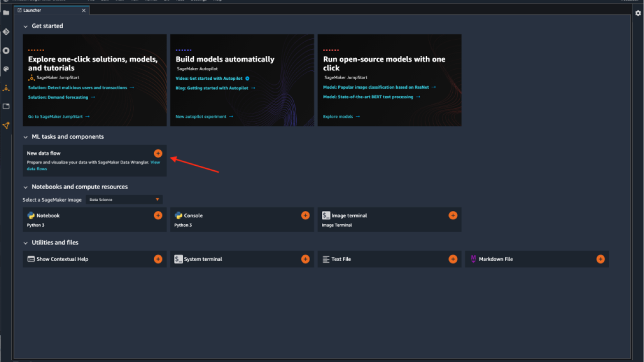
2. When Studio opens, choose the plus sign on the New data flow card under ML tasks and components.

This creates a new directory in Studio with a .flow file inside, which contains your data flow. The .flow file automatically opens in Studio.

You can also create a new flow by choosing File, then New, and choosing Data Wrangler Flow.

3. Optionally, rename the new directory and the .flow file.

When you create a new .flow file in Studio, you might see a carousel that introduces you to Data Wrangler. This may take a few minutes.

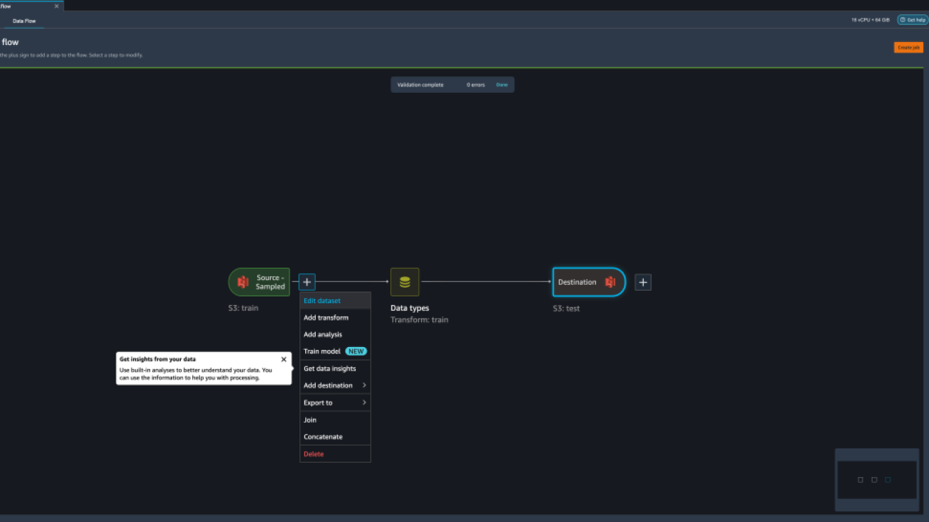
When the Data Wrangler instance is active, you can see the data flow screen as shown in the following screenshot.

4. Choose Use sample dataset to load the titanic dataset.

Create a Quick Model analysis

There are two ways to get a sense for a new (previously unseen) dataset. One is to run Data Quality and Insights Report. This report will provide high level statistics – number features, rows, missing values, etc and surface high priority warnings (if present) – duplicate rows, target leakage, anomalous samples, etc.

Another way is to run Quick Model analysis directly. Complete the following steps:

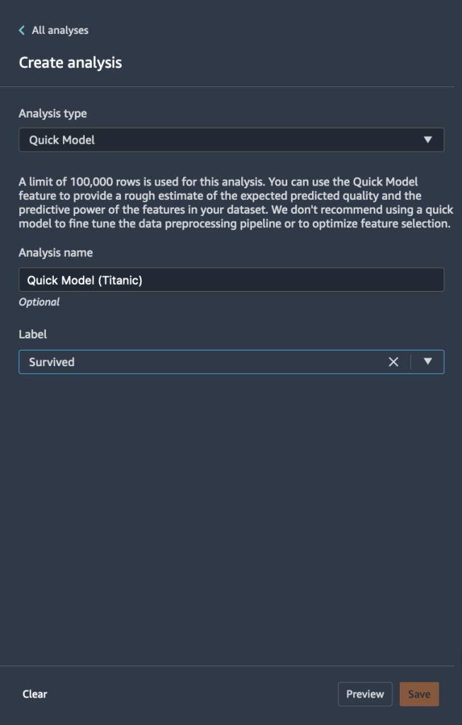
1. Choose the plus sign and choose Add analysis.

2. For Analysis type, choose Quick Model.
3. For Analysis name¸ enter a name.
4. For Label, choose the target label from the list of your feature columns (Survived).
5. Choose Save.

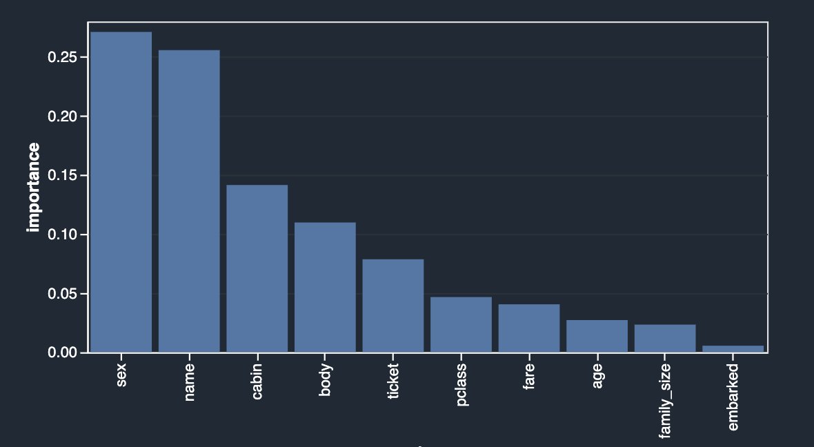
The following graph visualizes our findings.

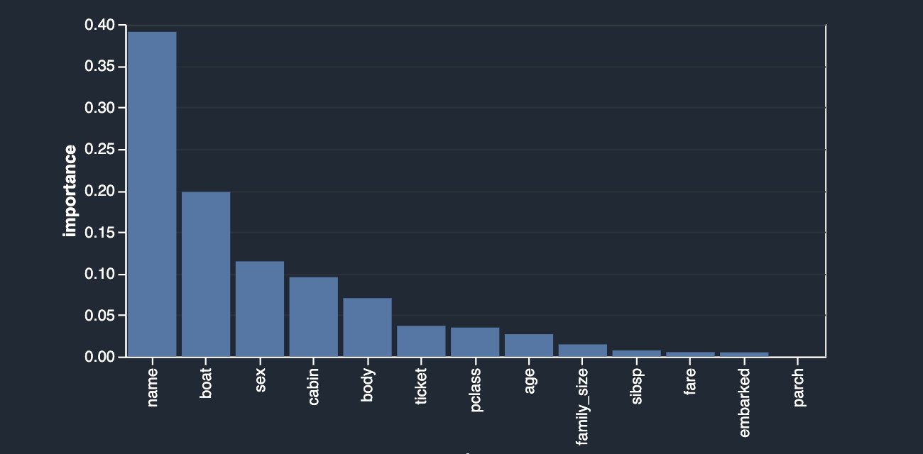
Quick Model trains a random forest with 10 trees on 730 observations and measures prediction quality on the remaining 315 observations. The dataset is automatically sampled and split into training and validation tests (70:30). In this example, you can see that the model achieved an F1 score of 0.777 on the test set. This could be an indicator that the data you’re exploring has the potential of being predictive.

At the same time, a few things stand out right away. The columns name and boat are the highest contributing signals towards your prediction. String columns like name can be both useful and not useful depending on the comprehensive information they carry about the person, like first, middle, and last names alongside the historical time periods and trends they belong to. This column can either be excluded or retained depending on the outcome of the contribution. In this case, a simple preview reveals that passenger names also include their titles (Mr, Dr, etc) which could potentially carry valuable information; therefore, we’re going to keep it. However, we do want to take a closer look at the boat column, which also seems to have a strong predictive power.

Target leakage

First, let’s start with the concept of leakage. Leakage can occur during different stages of the ML lifecycle. Using features that are available only during training but not during inference can also be defined as target leakage. For example, a deployed airbag is not a good predictor for a car crash, because in real life it occurs after the fact.

One of the techniques for identifying target leakage relies on computing ROC values for each feature. The closer the value is to a 1, the more likely the feature is very predictive of the target and therefore the more likely it’s a leaked target. On the other hand, the closer the value is to 0.5 and below (rarely), the less likely this feature contributes anything towards prediction. Finally, values that are above 0.5 and below 1 indicate that the feature doesn’t carry predictive power by itself, but may be a contributor in a group—which is what we’d like to see ideally.

Let’s create a target leakage analysis on your dataset. This analysis together with a set of advanced analyses are offered as built-in analysis types in Data Wrangler. To create the analysis, choose Add Analysis and choose Target Leakage. This is similar to how you previously created a Quick Model analysis.

As you can see in the following figure, your most predictive feature boat is quite close in ROC value to 1, which makes it a possible suspect for target leakage.

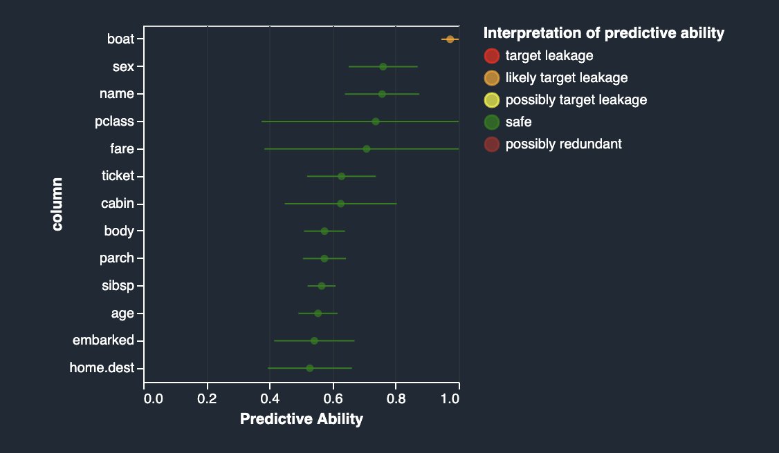
If you read the description of the dataset, the boat column contains the lifeboat number in which the passenger managed to escape. Naturally, there is quite a close correlation with the survival label. The lifeboat number is known only after the fact—when the lifeboat was picked up and the survivors on it were identified. This is very similar to the airbag example. Therefore, the boat column is indeed a target leakage.

You can eliminate it from your dataset by applying the drop column transform in the Data Wrangler UI (choose Handle Columns, choose Drop, and indicate boat). Now if you rerun the analysis, you get the following.

Multicollinearity

Multicollinearity occurs when two or more features in a dataset are highly correlated with one another. Detecting the presence of multicollinearity in a dataset is important because multicollinearity can reduce predictive capabilities of an ML model. Multicollinearity can either already be present in raw data received from an upstream system, or it can be inadvertently introduced during feature engineering. For instance, the Titanic dataset contains two columns indicating the number of family members each passenger traveled with: number of siblings (sibsp) and number of parents (parch). Let’s say that somewhere in your feature engineering pipeline, you decided that it would make sense to introduce a simpler measure of each passenger’s family size by combining the two.

A very simple transformation step can help us achieve that, as shown in the following screenshot.

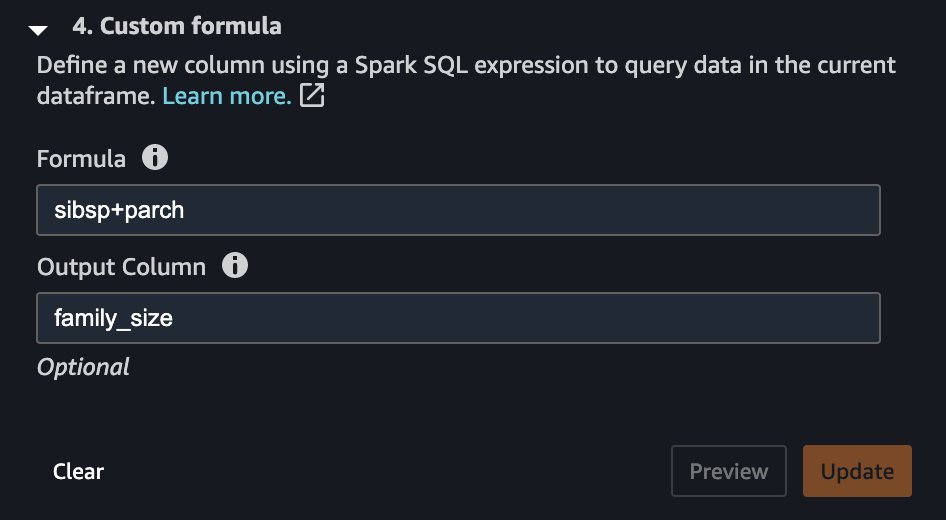
As a result, you now have a column called family_size, which reflects just that. If you didn’t drop the original two columns, you now have very strong correlation between both siblings as well as the parents columns and the family size. By creating another analysis and choosing Multicollinearity, you can now see the following.

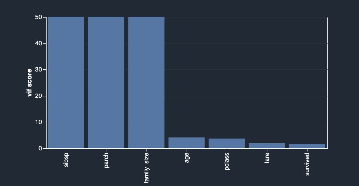
In this case, you’re using the Variance Inflation Factor (VIF) approach to identify highly correlated features. VIF scores are calculated by solving a regression problem to predict one variable given the rest, and they can range between 1 and infinity. The higher the value is, the more dependent a feature is. Data Wrangler’s implementation of VIF analysis caps the scores at 50 and in general, a score of 5 means the feature is moderately correlated, whereas anything above 5 is considered highly correlated.

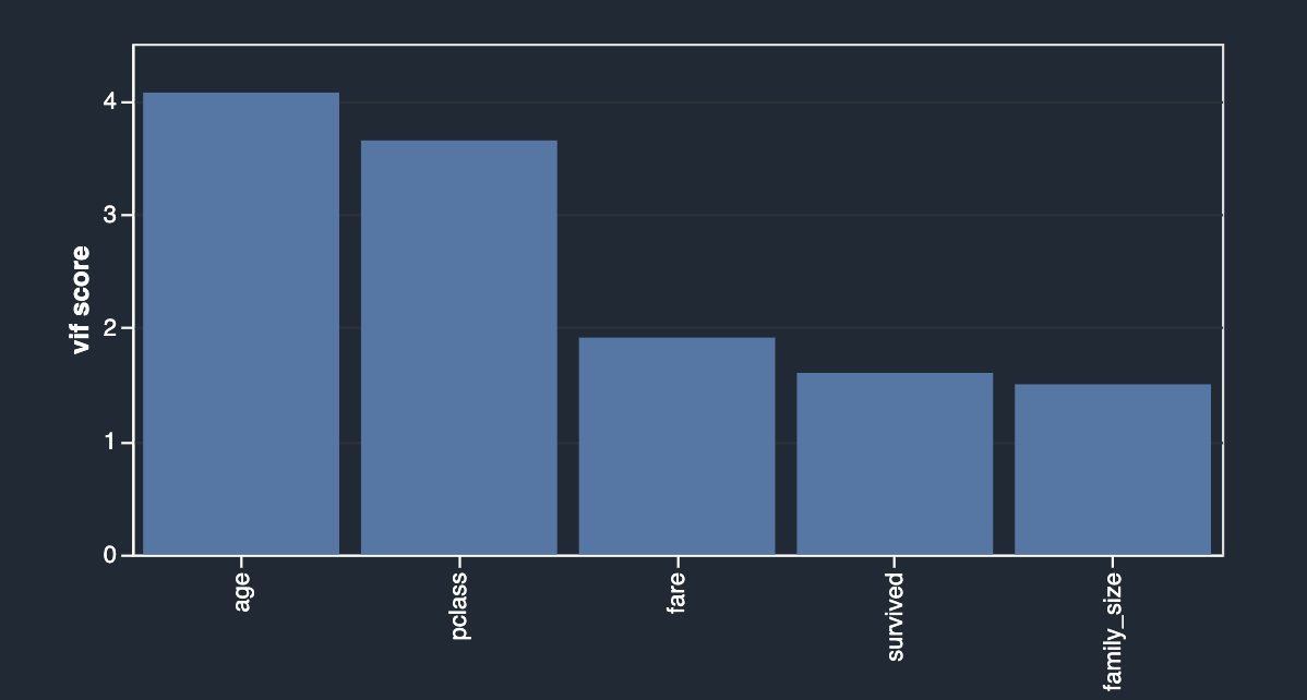
Your newly engineered feature is highly dependent on the original columns, which you can now simply drop by using another transformation by choosing Manage Columns, Drop Column.

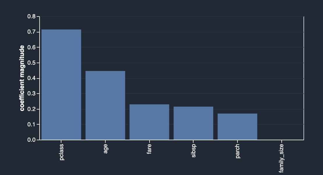
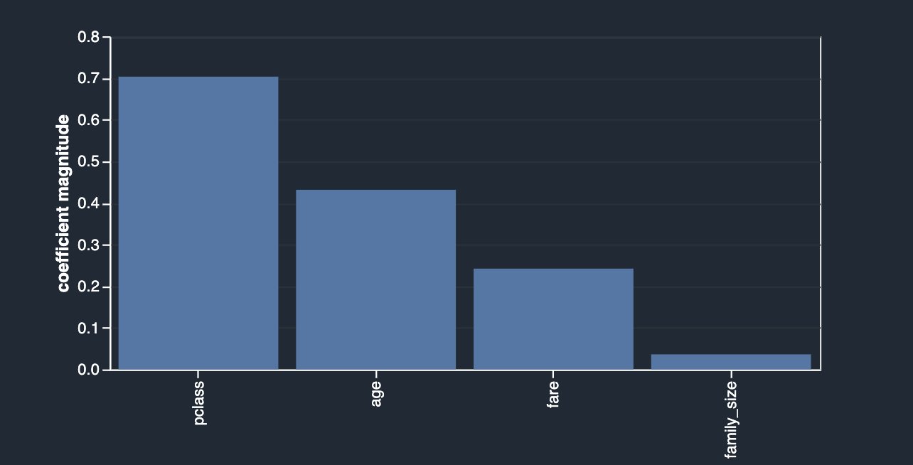
An alternative approach to identify features that have less or more predictive power is to use the Lasso feature selection type of the multicollinearity analysis (for Problem type, choose Classification and for Label column, choose survived).

As outlined in the description, this analysis builds a linear classifier that provides a coefficient for each feature. The absolute value of this coefficient can also be interpreted as the importance score for the feature. As you can observe in your case, family_size carries no value in terms of feature importance due to its redundancy, unless you drop the original columns.

After dropping sibsp and parch, you get the following.

Data Wrangler also provides a third option to detect multicollinearity in your dataset facilitated via Principal Component Analysis (PCA). PCA measures the variance of the data along different directions in the feature space. The ordered list of variances, also known as the singular values, can inform about multicollinearity in your data. This list contains non-negative numbers. When the numbers are roughly uniform, the data has very few multicollinearities. However, when the opposite is true, the magnitude of the top values will dominate the rest. To avoid issues related to different scales, the individual features are standardized to have mean 0 and standard deviation 1 before applying PCA.

Before dropping the original columns (sibsp and parch), your PCA analysis is shown as follows.

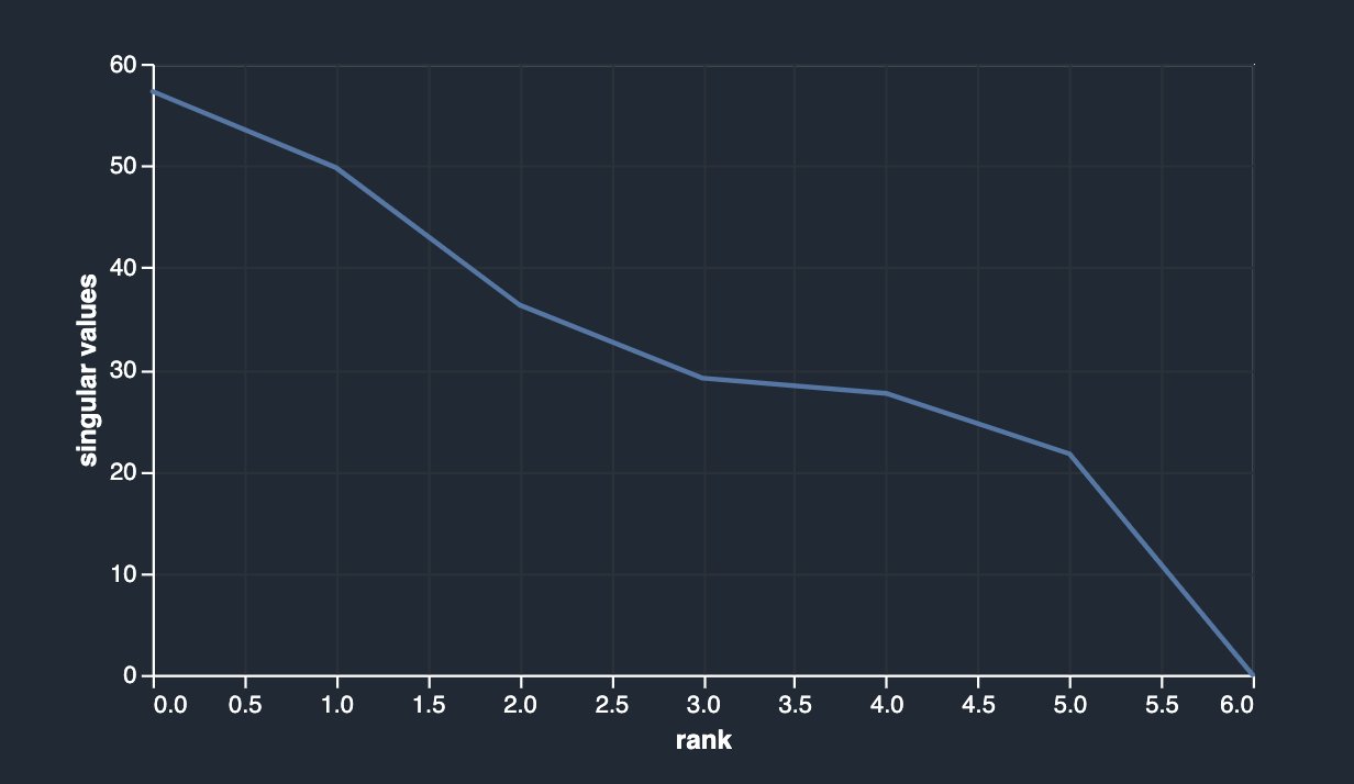
After dropping sibsp and parch, you have the following.

Feature correlation

Correlation is a measure of the degree of dependence between variables. Correlated features in general don’t improve models but can have an impact on models. There are two types of correlation detection features available in Data Wrangler: linear and non-linear.

Linear feature correlation is based on Pearson’s correlation. Numeric-to-numeric correlation is in the range [-1, 1] where 0 implies no correlation, 1 implies perfect correlation, and -1 implies perfect inverse correlation. Numeric-to-categorical and categorical-to-categorical correlations are in the range [0, 1] where 0 implies no correlation and 1 implies perfect correlation. Features that are not either numeric or categorical are ignored.

The following correlation matrix and score table validate and reinforce your previous findings.

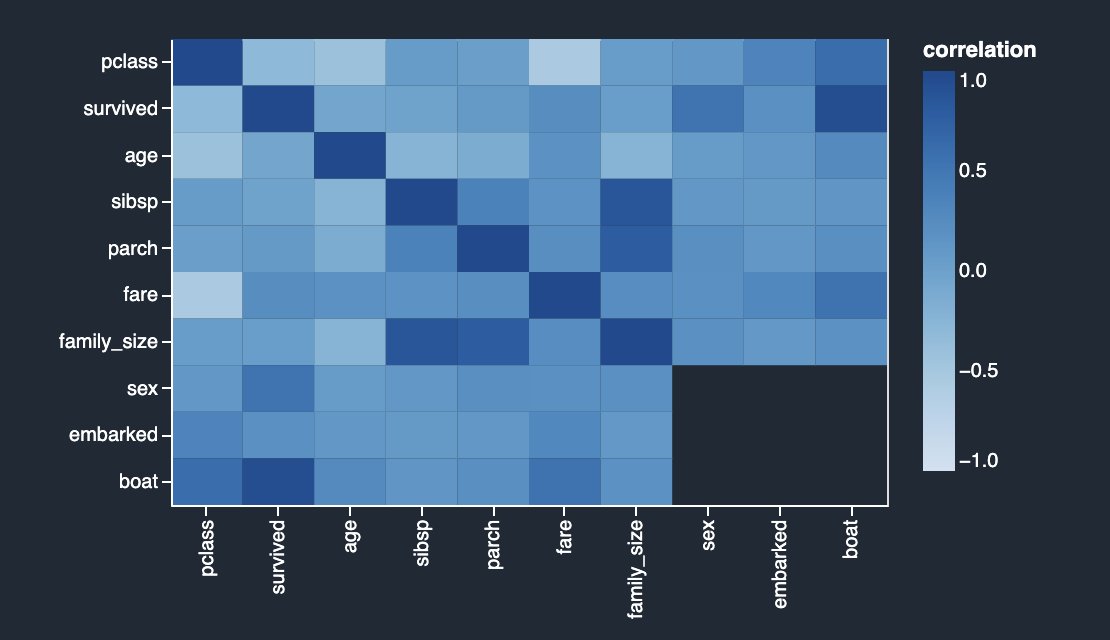
The columns survived and boat are highly correlating with each other. For this example, survived is the target column or the label you’re trying to predict. You saw this previously in your target leakage analysis. On the other hand, columns sibsp and parch are highly correlating with the derived feature family_size. This was confirmed in your previous multicollinearity analysis. We don’t see any strong inverse linear correlation in the dataset.

When two variable changes in a constant proportion, it’s called a linear correlation, whereas when the two variables don’t change in any constant proportion, the relationship is non-linear. Correlation is perfectly positive when proportional change in two variables is in the same direction. In contrast, correlation is perfectly negative when proportional change in two variables is in the opposite direction.

The difference between feature correlation and multi-collinearity (discussed previously) is as follows: feature correlation refers to the linear or non-linear relationship between two variables. With this context, you can define collinearity as a problem where two or more independent variables (predictors) have a strong linear or non-linear relationship. Multicollinearity is a special case of collinearity where a strong linear relationship exists between three or more independent variables even if no pair of variables has a high correlation.

Non-linear feature correlation is based on Spearman’s rank correlation. Numeric-to-categorical correlation is calculated by encoding the categorical features as the floating-point numbers that best predict the numeric feature before calculating Spearman’s rank correlation. Categorical-to-categorical correlation is based on the normalized Cramer’s V test.

Numeric-to-numeric correlation is in the range [-1, 1] where 0 implies no correlation, 1 implies perfect correlation, and -1 implies perfect inverse correlation. Numeric-to-categorical and categorical-to-categorical correlations are in the range [0, 1] where 0 implies no correlation and 1 implies perfect correlation. Features that aren’t numeric or categorical are ignored.

The following table lists for each feature what is the most correlated feature to it. It displays a correlation matrix for a dataset with up to 20 columns.

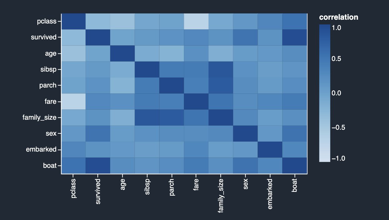
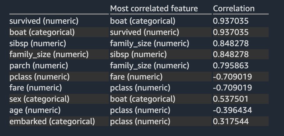
The results are very similar to what you saw in the previous linear correlation analysis, except you can also see a strong negative non-linear correlation between the pclass and fare numeric columns.

Finally, now that you have identified potential target leakage and eliminated features based on your analyses, let’s rerun the Quick Model analysis to look at the feature importance breakdown again.

The results look quite different than what you started with initially. Therefore, Data Wrangler makes it easy to run advanced ML-specific analysis with a few clicks and derive insights about the relationship between your independent variables (features) among themselves and also with the target variable. It also provides you with the Quick Model analysis type that lets you validate the current state of features by training a quick model and testing how predictive the model is.

Ideally, as a data scientist, you should start with some of the analyses showcased in this post and derive insights into what features are good to retain vs. what to drop.

Summary

In this post, you learned how to use Data Wrangler for exploratory data analysis, focusing on target leakage, feature correlation, and multicollinearity analyses to identify potential issues with training data and mitigate them with the help of built-in transformations. As next steps, we recommend you replicate the example in this post in your Data Wrangler data flow to experience what was discussed here in action.

If you’re new to Data Wrangler or Studio, refer to Get Started with Data Wrangler. If you have any questions related to this post, please add it in the comments section.

About the authors

Vadim Omeltchenko is a Sr. AI/ML Solutions Architect who is passionate about helping AWS customers innovate in the cloud. His prior IT experience was predominantly on the ground.

Arunprasath Shankar is a Sr. AI/ML Specialist Solutions Architect with AWS, helping global customers scale their AI solutions effectively and efficiently in the cloud. In his spare time, Arun enjoys watching sci-fi movies and listening to classical music.

Read More

At AWS, we have been investing in healthcare since Day 1 with customers including Moderna, Rush University Medical Center, and the NHS who have built breakthrough innovations in the cloud. From developing public health analytics hubs, to improving health equity and patient outcomes, to developing a COVID-19 vaccine in just 65 days, our customers are utilizing machine learning (ML) and the cloud to address some of healthcare’s biggest challenges and drive change toward more predictive and personalized care.

Last year, we launched Amazon HealthLake, a purpose-built service to store, transform, and query health data in the cloud, allowing you to benefit from a complete view of individual or patient population health data at scale.

Today, we’re excited to announce the launch of two new capabilities in HealthLake that deliver innovations for medical imaging and analytics.

Amazon HealthLake Imaging

Healthcare professionals face a myriad of challenges as the scale and complexity of medical imaging data continues to increase including the following:

• The volume of medical imaging data has continued to accelerate over the past decade with over 5.5 billion imaging procedures done across the globe each year by a shrinking number of radiologists
• The average imaging study size has doubled over the past decade to 150 MB as more advanced imaging procedures are being performed due to improvements in resolution and the increasing use of volumetric imaging
• Health systems store multiple copies of the same imaging data in clinical and research systems, which leads to increased costs and complexity
• It can be difficult to structure this data, which often takes data scientists and researchers weeks or months to derive important insights with advanced analytics and ML

These compounding factors are slowing down decision-making, which can affect care delivery. To address these challenges, we are excited to announce the preview of Amazon HealthLake Imaging, a new HIPAA-eligible capability that makes it easy to store, access, and analyze medical images at petabyte scale. This new capability is designed for fast, sub-second  medical image retrieval in your clinical workflows that you can access securely from anywhere (e.g., web, desktop, phone) and with high availability. Additionally, you can drive your existing medical viewers and analysis applications from a single encrypted copy of the same data in the cloud with normalized metadata and advanced compression. As a result, it is estimated that HealthLake Imaging helps you reduce the total cost of medical imaging storage by up to 40%.

We are proud to be working with partners on the launch of HealthLake Imaging to accelerate adoption of cloud-native solutions to help transition enterprise imaging workflows to the cloud and accelerate your pace of innovation.

Intelerad and Arterys are among the launch partners utilizing HealthLake Imaging to achieve higher scalability and viewing performance for their next-generation PACS systems and AI platform, respectively. Radical Imaging is providing customers with zero-footprint, cloud-capable medical imaging applications using open-source projects, such as OHIF or Cornerstone.js, built on HealthLake Imaging APIs. And NVIDIA has collaborated with AWS to develop a MONAI connector for HealthLake Imaging. MONAI is an open-source medical AI framework to develop and deploy models into AI applications, at scale.

“Intelerad has always focused on solving complex problems in healthcare, while enabling our customers to grow and provide exceptional patient care to more patients around the globe. In our continuous path of innovation, our collaboration with AWS, including leveraging Amazon HealthLake Imaging, allows us to innovate more quickly and reduce complexity while offering unparalleled scale and performance for our users.”

— AJ Watson, Chief Product Officer at Intelerad Medical Systems

“With Amazon HealthLake Imaging, Arterys was able to achieve noticeable improvements in performance and responsiveness of our applications, and with a rich feature set of future-looking enhancements, offers benefits and value that will enhance solutions looking to drive future-looking value out of imaging data.”

— Richard Moss, Director of Product Management at Arterys

Radboudumc and the University of Maryland Medical Intelligent Imaging Center (UM2ii) are among the customers utilizing HealthLake Imaging to improve the availability of medical images and utilize image streaming.

“At Radboud University Medical Center, our mission is to be a pioneer in shaping a more person-centered, innovative future of healthcare. We are building a collaborative AI solution with Amazon HealthLake Imaging for clinicians and researchers to speed up innovation by putting ML algorithms into the hands of clinicians faster.”

— Bram van Ginneken, Chair, Diagnostic Image Analysis Group at Radboudumc

“UM2ii was formed to unite innovators, thought leaders, and scientists across academics and industry. Our work with AWS will accelerate our mission to push the boundaries of medical imaging AI. We are excited to build the next generation of cloud-based intelligent imaging with Amazon HealthLake Imaging and AWS’s experience with scalability, performance, and reliability.”

— Paul Yi, Director at UM2ii

Amazon HealthLake Analytics

The second capability we’re excited to announce is Amazon HealthLake Analytics. Harnessing multi-modal data, which is highly contextual and complex, is key to making meaningful progress in providing patients highly personalized and precisely targeted diagnostics and treatments.

HealthLake Analytics makes it easy to query and derive insights from multi-modal health data at scale, at the individual or population levels, with the ability to share data securely across the enterprise and enable advanced analytics and ML in just a few clicks. This removes the need for you to execute complex data exports and data transformations.

HealthLake Analytics automatically normalizes raw health data from multiple disparate sources (e.g. medical records, health insurance claims, EHRs, medical devices) into an analytics and interoperability-ready format in a matter of minutes. Integration with other AWS services makes it easy to query the data with SQL using Amazon Athena, as well as share and analyze data to enable advanced analytics and ML. You can create powerful dashboards with Amazon QuickSight for care gap analyses and disease management of an entire patient population. Or you can build and train many ML models quickly and efficiently in Amazon SageMaker for AI-driven predictions, such as risk of hospital readmission or overall effectiveness of a line of treatment. HealthLake Analytics reduces what would take months of engineering effort and allows you to do what you do best—deliver care for patients.

Conclusion

At AWS, our goal is to support you to deliver convenient, personalized, and high-value care – helping you to reinvent how you collaborate, make data-driven clinical and operational decisions, enable precision medicine, accelerate therapy development, and decrease the cost of care.

With these new capabilities in Amazon HealthLake, we along with our partners can help enable next-generation imaging workflows in the cloud and derive insights from multi-modal health data, while complying with HIPAA, GDPR, and other regulations.

To learn more and get started, refer to Amazon HealthLake Analytics and Amazon HealthLake Imaging.

About the authors

Tehsin Syed is General Manager of Health AI at Amazon Web Services, and leads our Health AI engineering and product development efforts including Amazon Comprehend Medical and Amazon Health. Tehsin works with teams across Amazon Web Services responsible for engineering, science, product and technology to develop ground breaking healthcare and life science AI solutions and products. Prior to his work at AWS, Tehsin was Vice President of engineering at Cerner Corporation where he spent 23 years at the intersection of healthcare and technology.

Dr. Taha Kass-Hout is Vice President, Machine Learning, and Chief Medical Officer at Amazon Web Services, and leads our Health AI strategy and efforts, including Amazon Comprehend Medical and Amazon HealthLake. He works with teams at Amazon responsible for developing the science, technology, and scale for COVID-19 lab testing, including Amazon’s first FDA authorization for testing our associates—now offered to the public for at-home testing. A physician and bioinformatician, Taha served two terms under President Obama, including the first Chief Health Informatics officer at the FDA. During this time as a public servant, he pioneered the use of emerging technologies and the cloud (the CDC’s electronic disease surveillance), and established widely accessible global data sharing platforms: the openFDA, which enabled researchers and the public to search and analyze adverse event data, and precisionFDA (part of the Presidential Precision Medicine initiative).

Read More