Monthly Archives: November 2022

Amazon SageMaker Data Wrangler helps you understand, aggregate, transform, and prepare data for machine learning (ML) from a single visual interface. It contains over 300 built-in data transformations so you can quickly normalize, transform, and combine features without having to write any code.

Data science practitioners generate, observe, and process data to solve business problems where they need to transform and extract features from datasets. Transforms such as ordinal encoding or one-hot encoding learn encodings on your dataset. These encoded outputs are referred as trained parameters. As datasets change over time, it may be necessary to refit encodings on previously unseen data to keep the transformation flow relevant to your data.

We are excited to announce the refit trained parameter feature, which allows you to use previous trained parameters and refit them as desired. In this post, we demonstrate how to use this feature.

Overview of the Data Wrangler refit feature

We illustrate how this feature works with the following example, before we dive into the specifics of the refit trained parameter feature.

Assume your customer dataset has a categorical feature for country represented as strings like Australia and Singapore. ML algorithms require numeric inputs; therefore, these categorical values have to be encoded to numeric values. Encoding categorical data is the process of creating a numerical representation for categories. For example, if your category country has values Australia and Singapore, you may encode this information into two vectors: [1, 0] to represent Australia and [0, 1] to represent Singapore. The transformation used here is one-hot encoding and the new encoded output reflects the trained parameters.

After training the model, over time your customers may increase and you have more distinct values in the country list. The new dataset could contain another category, India, which wasn’t part of the original dataset, which can affect the model accuracy. Therefore, it’s necessary to retrain your model with the new data that has been collected over time.

To overcome this problem, you need to refresh the encoding to include the new category and update the vector representation as per your latest dataset. In our example, the encoding should reflect the new category for the country, which is India. We commonly refer to this process of refreshing an encoding as a refit operation. After you perform the refit operation, you get the new encoding: Australia: [1, 0, 0], Singapore: [0, 1, 0], and India: [0, 0, 1]. Refitting the one-hot encoding and then retraining the model on the new dataset results in better quality predictions.

Data Wrangler’s refit trained parameter feature is useful in the following cases:

• New data is added to the dataset – Retraining the ML model is necessary when the dataset is enriched with new data. To achieve optimal results, we need to refit the trained parameters on the new dataset.
• Training on a full dataset after performing feature engineering on sample data – For a large dataset, a sample of the dataset is considered for learning trained parameters, which may not represent your entire dataset. We need to relearn the trained parameters on the complete dataset.

The following are some of the most common Data Wrangler transforms performed on the dataset that benefit from the refit trained parameter option:

• Encode categorical
• Featurize text
• Process numeric
• Handling outliers

For more information about transformations in Data Wrangler, refer to Transform Data.

In this post, we show how to process these trained parameters on datasets using Data Wrangler. You can use Data Wrangler flows in production jobs to reprocess your data as it grows and changes.

Solution overview

For this post, we demonstrate how to use the Data Wrangler’s refit trained parameter feature with the publicly available dataset on Kaggle: US Housing Data from Zillow, For-Sale Properties in the United States. It has the home sale prices across various geo-distributions of homes.

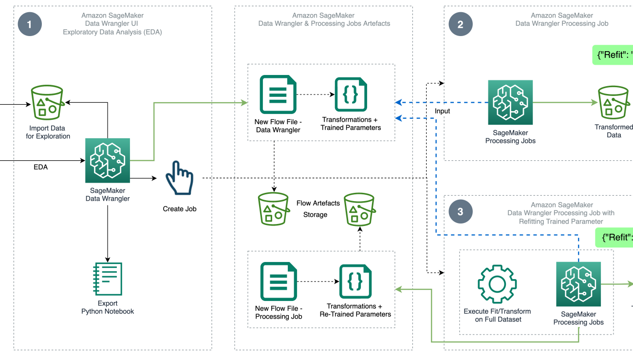
The following diagram illustrates the high-level architecture of Data Wrangler using the refit trained parameter feature. We also show the effect on the data quality without the refit trained parameter and contrast the results at the end.

The workflow includes the following steps:

1. Perform exploratory data analysis – Create a new flow on Data Wrangler to start the exploratory data analysis (EDA). Import business data to understand, clean, aggregate, transform, and prepare your data for training. Refer to Explore Amazon SageMaker Data Wrangler capabilities with sample datasets for more details on performing EDA with Data Wrangler.
2. Create a data processing job – This step exports all the transformations that you made on the dataset as a flow file stored in the configured Amazon Simple Storage Service (Amazon S3) location. The data processing job with the flow file generated by Data Wrangler applies the transforms and trained parameters learned on your dataset. When the data processing job is complete, the output files are uploaded to the Amazon S3 location configured in the destination node. Note that the refit option is turned off by default. As an alternative to executing the processing job instantly, you can also schedule a processing job in a few clicks using Data Wrangler – Create Job to run at specific times.
3. Create a data processing job with the refit trained parameter feature – Select the new refit trained parameter feature while creating the job to enforce relearning of your trained parameters on your full or reinforced dataset. As per the Amazon S3 location configuration for storing the flow file, the data processing job creates or updates the new flow file. If you configure the same Amazon S3 location as in Step 2, the data processing job updates the flow file generated in the Step 2, which can be used to keep your flow relevant to your data. On completion of the processing job, the output files are uploaded to the destination node configured S3 bucket. You can use the updated flow on your entire dataset for a production workflow.

Prerequisites

Before getting started, upload the dataset to an S3 bucket, then import it into Data Wrangler. For instructions, refer to Import data from Amazon S3.

Let’s now walk through the steps mentioned in the architecture diagram.

Perform EDA in Data Wrangler

To try out the refit trained parameter feature, set up the following analysis and transformation in Data Wrangler. At the end of setting up EDA, Data Wrangler creates a flow file captured with trained parameters from the dataset.

1. Create a new flow in Amazon SageMaker Data Wrangler for exploratory data analysis.
2. Import the business data you uploaded to Amazon S3.
3. You can preview the data and options for choosing the file type, delimiter, sampling, and so on. For this example, we use the First K sampling option provided by Data Wrangler to import first 50,000 records from the dataset.
4. Choose Import.

5. After you check out the data type matching applied by Data Wrangler, add a new analysis.

6. For Analysis type, choose Data Quality and Insights Report.
7. Choose Create.

With the Data Quality and Insights Report, you get a brief summary of the dataset with general information such as missing values, invalid values, feature types, outlier counts, and more. You can pick features property_type and city for applying transformations on the dataset to understand the refit trained parameter feature.

Let’s focus on the feature property_type from the dataset. In the report’s Feature Details section, you can see the property_type, which is a categorical feature, and six unique values derived from the 50,000 sampled dataset by Data Wrangler. The complete dataset may have more categories for the feature property_type. For a feature with many unique values, you may prefer ordinal encoding. If the feature has a few unique values, a one-hot encoding approach can be used. For this example, we opt for one-hot encoding on property_type.

Similarly, for the city feature, which is a text data type with a large number of unique values, let’s apply ordinal encoding to this feature.

8. Navigate to the Data Wrangler flow, choose the plus sign, and choose Add transform.

9. Choose the Encode categorical option for transforming categorical features.

From the Data Quality and Insights Report, feature property_type shows six unique categories: CONDO, LOT, MANUFACTURED, SINGLE_FAMILY, MULTI_FAMILY, and TOWNHOUSE.

10. For Transform, choose One-hot encode.

After applying one-hot encoding on feature property_type, you can preview all six categories as separate features added as new columns. Note that 50,000 records were sampled from your dataset to generate this preview. While running a Data Wrangler processing job with this flow, these transformations are applied to your entire dataset.

11. Add a new transform and choose Encode Categorical to apply a transform on the feature city, which has a larger number of unique categorical text values.
12. To encode this feature into a numeric representation, choose Ordinal encode for Transform.

13. Choose Preview on this transform.

You can see that the categorical feature city is mapped to ordinal values in the output column e_city.

14. Add this step by choosing Update.

15. You can set the destination to Amazon S3 to store the applied transformations on the dataset to generate the output as CSV file.

Data Wrangler stores the workflow you defined in the user interface as a flow file and uploads to the configured data processing job’s Amazon S3 location. This flow file is used when you create Data Wrangler processing jobs to apply the transforms on larger datasets, or to transform new reinforcement data to retrain the model.

Launch a Data Wrangler data processing job without refit enabled

Now you can see how the refit option uses trained parameters on new datasets. For this demonstration, we define two Data Wrangler processing jobs operating on the same data. The first processing job won’t enable refit; for the second processing job, we use refit. We compare the effects at the end.

1. Choose Create job to initiate a data processing job with Data Wrangler.

2. For Job name, enter a name.
3. Under Trained parameters, do not select Refit.
4. Choose Configure job.

5. Configure the job parameters like instance types, volume size, and Amazon S3 location for storing the output flow file.
6. Data Wrangler creates a flow file in the flow file S3 location. The flow uses transformations to train parameters, and we later use the refit option to retrain these parameters.
7. Choose Create.

Wait for the data processing job to complete to see the transformed data in the S3 bucket configured in the destination node.

Launch a Data Wrangler data processing job with refit enabled

Let’s create another processing job enabled with the refit trained parameter feature enabled. This option enforces the trained parameters relearned on the entire dataset. When this data processing job is complete, a flow file is created or updated to the configured Amazon S3 location.

1. Choose Create job.

2. For Job name, enter a name.
3. For Trained parameters, select Refit.
4. If you choose View all, you can review all the trained parameters.

5. Choose Configure job.
6. Enter the Amazon S3 flow file location.
7. Choose Create.

Wait for the data processing job to complete.

Refer to the configured S3 bucket in the destination node to view the data generated by the data processing job running the defined transforms.

Export to Python code for running Data Wrangler processing jobs

As an alternative to starting the processing jobs using the Create job option in Data Wrangler, you can trigger the data processing jobs by exporting the Data Wrangler flow to a Jupyter notebook. Data Wrangler generates a Jupyter notebook with inputs, outputs, processing job configurations, and code for job status checks. You can change or update the parameters as per your data transformation requirements.

1. Choose the plus sign next to the final Transform node.
2. Choose Export to and Amazon S3 (Via Jupyter Notebook).

You can see a Jupyter notebook opened with inputs, outputs, processing job configurations, and code for job status checks.

3. To enforce the refit trained parameters option via code, set the refit parameter to True.

Compare data processing job results

After the Data Wrangler processing jobs are complete, you must create two new Data Wrangler flows with the output generated by the data processing jobs stored in the configured Amazon S3 destination.

You can refer to the configured location in the Amazon S3 destination folder to review the data processing jobs’ outputs.

To inspect the processing job results, create two new Data Wrangler flows using the Data Quality and Insights Report to compare the transformation results.

1. Create a new flow in Amazon SageMaker Data Wrangler.
2. Import the data processing job without refit enabled output file from Amazon S3.
3. Add a new analysis.
4. For Analysis type, choose Data Quality and Insights Report.
5. Choose Create.

Repeat the above steps and create new data wrangler flow to analyze the data processing job output with refit enabled.

Now let’s look at the outputs of processing jobs for the feature property_type using the Data Quality and Insights Reports. Scroll to the feature details on the Data and Insights Reports listing feature_type.

The refit trained parameter processing job has refitted the trained parameters on the entire dataset and encoded the new value APARTMENT with seven distinct values on the full dataset.

The normal processing job applied the sample dataset trained parameters, which have only six distinct values for the property_type feature. For data with feature_type APARTMENT, the invalid handling strategy Skip is applied and the data processing job doesn’t learn this new category. The one-hot encoding has skipped this new category present on the new data, and the encoding skips the category APARTMENT.

Let’s now focus on another feature, city. The refit trained parameter processing job has relearned all the values available for the city feature, considering the new data.

As shown in the Feature Summary section of the report, the new encoded feature column e_city has 100% valid parameters by using the refit trained parameter feature.

In contrast, the normal processing job has 82.4% of missing values in the new encoded feature column e_city. This phenomenon is because only the sample set of learned trained parameters are applied on the full dataset and no refitting is applied by the data processing job.

The following histograms depict the ordinal encoded feature e_city. The first histogram is of the feature transformed with the refit option.

The next histogram is of the feature transformed without the refit option. The orange column shows missing values (NaN) in the Data Quality and Insights Report. The new values that aren’t learned from the sample dataset are replaced as Not a Number (NaN) as configured in the Data Wrangler UI’s invalid handling strategy.

The data processing job with the refit trained parameter relearned the property_type and city features considering the new values from the entire dataset. Without the refit trained parameter, the data processing job only uses the sampled dataset’s pre-learned trained parameters. It then applies them to the new data, but the new values aren’t considered for encoding. This will have implications on the model accuracy.

Clean up

When you’re not using Data Wrangler, it’s important to shut down the instance on which it runs to avoid incurring additional fees.

To avoid losing work, save your data flow before shutting Data Wrangler down.

1. To save your data flow in Amazon SageMaker Studio, choose File, then choose Save Data Wrangler Flow. Data Wrangler automatically saves your data flow every 60 seconds.
2. To shut down the Data Wrangler instance, in Studio, choose Running Instances and Kernels.
3. Under RUNNING APPS, choose the shutdown icon next to the sagemaker-data-wrangler-1.0 app.

4. Choose Shut down all to confirm.

Data Wrangler runs on an ml.m5.4xlarge instance. This instance disappears from RUNNING INSTANCES when you shut down the Data Wrangler app.

After you shut down the Data Wrangler app, it has to restart the next time you open a Data Wrangler flow file. This can take a few minutes.

Conclusion

In this post, we provided an overview of the refit trained parameter feature in Data Wrangler. With this new feature, you can store the trained parameters in the Data Wrangler flow, and the data processing jobs use the trained parameters to apply the learned transformations on large datasets or reinforcement datasets. You can apply this option to vectorizing text features, numerical data, and handling outliers.

Preserving trained parameters throughout the data processing of the ML lifecycle simplifies and reduces the data processing steps, supports robust feature engineering, and supports model training and reinforcement training on new data.

We encourage you to try out this new feature for your data processing requirements.

About the authors

Hariharan Suresh is a Senior Solutions Architect at AWS. He is passionate about databases, machine learning, and designing innovative solutions. Prior to joining AWS, Hariharan was a product architect, core banking implementation specialist, and developer, and worked with BFSI organizations for over 11 years. Outside of technology, he enjoys paragliding and cycling.

Santosh Kulkarni is an Enterprise Solutions Architect at Amazon Web Services who works with sports customers in Australia. He is passionate about building large-scale distributed applications to solve business problems using his knowledge in AI/ML, big data, and software development.

Vishaal Kapoor is a Senior Applied Scientist with AWS AI. He is passionate about helping customers understand their data in Data Wrangler. In his spare time, he mountain bikes, snowboards, and spends time with his family.

Aniketh Manjunath is a Software Development Engineer at Amazon SageMaker. He helps support Amazon SageMaker Data Wrangler and is passionate about distributed machine learning systems. Outside of work, he enjoys hiking, watching movies, and playing cricket.

Read More

Today, we are launching Amazon SageMaker inference on AWS Graviton to enable you to take advantage of the price, performance, and efficiency benefits that come from Graviton chips.

Graviton-based instances are available for model inference in SageMaker. This post helps you migrate and deploy a machine learning (ML) inference workload from x86 to Graviton-based instances in SageMaker. We provide a step-by-step guide to deploy your SageMaker trained model to Graviton-based instances, cover best practices when working with Graviton, discuss the price-performance benefits, and demo how to deploy a TensorFlow model on a SageMaker Graviton instance.

Brief overview of Graviton

AWS Graviton is a family of processors designed by AWS that provide the best price-performance and are more energy efficient than their x86 counterparts. AWS Graviton 3 processors are the latest in the Graviton processor family and are optimized for ML workloads, including support for bfloat16, and twice the Single Instruction Multiple Data (SIMD) bandwidth. When these two features are combined, Graviton 3 can deliver up to three times better performance vs. Graviton 2 instances. Graviton 3 also uses up to 60% less energy for the same performance as comparable Amazon Elastic Compute Cloud (Amazon EC2) instances. This is a great feature if you want to reduce your carbon footprint and achieve your sustainability goals.

Solution overview

To deploy your models to Graviton instances, you either use AWS Deep Learning Containers or bring your own containers compatible with Arm v8.2 architecture.

The migration (or new deployment) of your models from x86 powered instances to Graviton instances is simple because AWS provides containers to host models with PyTorch, TensorFlow, Scikit-learn, and XGBoost, and the models are architecture agnostic. Nevertheless, if you’re willing to bring your own libraries, you can also do so, just ensure that your container is built with an environment that supports Arm64 architecture. For more information, see Building your own algorithm container.

You need to complete three steps to deploy your model:

1. Create a SageMaker model: This will contain, among other parameters, the information about the model file location, the container that will be used for the deployment, and the location of the inference script. (If you have an existing model already deployed in an x86 based inference instance, you can skip this step.)
2. Create an endpoint configuration: This will contain information about the type of instance you want for the endpoint (for example, ml.c7g.xlarge for Graviton3), the name of the model you created in the step 1, and the number of instances per endpoint.
3. Launch the endpoint with the endpoint configuration created in the step 2.

Prerequisites

Before starting, consider the following prerequisites:

1. Complete the prerequisites as listed in Prerequisites.
2. Your model should be either a PyTorch, TensorFlow, XGBoost, or Scikit-learn based model. The following table summarizes the versions currently supported as of this writing. For the latest updates, refer to SageMaker Framework Containers (SM support only).
   

   .	Python	TensorFlow	PyTorch	Scikit-learn	XGBoost
   Versions supported	3.8	2.9.1	1.12.1	1.0-1	1.3-1 to 1.5-1

3. The inference script is stored in Amazon Simple Storage Service (Amazon S3).

In the following sections, we walk you through the deployment steps.

Create a SageMaker model

If you have an existing model already deployed in an x86-based inference instance, you can skip this step. Otherwise, complete the following steps to create a SageMaker model:

1. Locate the model that you stored in an S3 bucket. Copy the URI.
   You use the model URI later in the MODEL_S3_LOCATION.
2. Identify the framework version and Python version that was used during model training.
   You need to select a container from the list of available AWS Deep Learning Containers per your framework and Python version. For more information, refer to Introducing multi-architecture container images for Amazon ECR.
3. Locate the inference Python script URI in the S3 bucket (the common file name is inference.py).
   The inference script URI is needed in the INFERENCE_SCRIPT_S3_LOCATION.
4. With these variables, you can then call the SageMaker API with the following command:

   client = boto3.client("sagemaker")
   
   client.create_model(
       ModelName="Your model name",
       PrimaryContainer={
           "Image": <AWS_DEEP_LEARNING_CONTAINER_URI>,
           "ModelDataUrl": <MODEL_S3_LOCATION>,
           "Environment": {
           "SAGEMAKER_PROGRAM": "inference.py",
           "SAGEMAKER_SUBMIT_DIRECTORY": <INFERENCE_SCRIPT_S3_LOCATION>,
           "SAGEMAKER_CONTAINER_LOG_LEVEL": "20",
           "SAGEMAKER_REGION": <REGION>
           }
       },
       ExecutionRoleArn= <ARN for AmazonSageMaker-ExecutionRole>
   )

You can also create multi-architecture images, and use the same image but with different tags. You can indicate on which architecture your instance will be deployed. For more information, refer to Introducing multi-architecture container images for Amazon ECR.

Create an endpoint config

After you create the model, you have to create an endpoint configuration by running the following command (note the type of instance we’re using):

client.create_endpoint_config(
    EndpointConfigName= <Your endpoint config name>,
    ProductionVariants=[
        {
         "VariantName": "v0",
         "ModelName": "Your model name",
         "InitialInstanceCount": 1,
         "InstanceType": "ml.c7g.xlarge",
        },
    ]
)

The following screenshot shows the endpoint configuration details on the SageMaker console.

Launch the endpoint

With the endpoint config created in the previous step, you can deploy the endpoint:

client.create_endpoint(
    EndpointName = "<Your endpoint name>",
    EndpointConfigName = "<Your endpoint config name>"
    )

Wait until your model endpoint is deployed. Predictions can be requested in the same way you request predictions for your endpoints deployed in x86-based instances.

The following screenshot shows your endpoint on the SageMaker console.

What is supported

SageMaker provides performance-optimized Graviton deep containers for TensorFlow and PyTorch frameworks. These containers support computer vision, natural language processing, recommendations, and generic deep and wide model-based inference use cases. In addition to deep learning containers, SageMaker also provides containers for classical ML frameworks such as XGBoost and Scikit-learn. The containers are binary compatible across c6g/m6g and c7g instances, therefore migrating the inference application from one generation to another is seamless.

C6g/m6g supports fp16 (half-precision float) and for compatible models provides equivalent or better performance compared to c5 instances. C7g substantially increases the ML performance by doubling the SIMD width and supporting bfloat-16 (bf16), which is the most cost-efficient platform for running your models.

Both c6g/m6g and c7g provide good performance for classical ML (for example, XGBoost) compared to other CPU instances in SageMaker. Bfloat-16 support on c7g allows efficient deployment of bf16 trained or AMP (Automatic Mixed Precision) trained models. The Arm Compute Library (ACL) backend on Graviton provides bfloat-16 kernels that can accelerate even the fp32 operators via fast math mode, without the model quantization.

Recommended best practices

On Graviton instances, every vCPU is a physical core. There is no contention for the common CPU resources (unlike SMT), and the workload performance scaling is linear with every vCPU addition. Therefore, it’s recommended to use batch inference whenever the use case allows. This will enable efficient use of the vCPUs by parallel processing the batch on each physical core. If the batch inference isn’t possible, the optimal instance size for a given payload is required to ensure OS thread scheduling overhead doesn’t outweigh the compute power that comes with the additional vCPUs.

TensorFlow comes with Eigen kernels by default, and it’s recommended to switch to OneDNN with ACL to get the most optimized inference backend. The OneDNN backend and the bfloat-16 fast math mode can be enabled while launching the container service:

docker run -p 8501:8501 --name tfserving_resnet 
--mount type=bind,source=/tmp/resnet,target=/models/resnet 
-e MODEL_NAME=resnet -e TF_ENABLE_ONEDNN_OPTS=1 
-e DNNL_DEFAULT_FPMATH_MODE=BF16 -e -t tfs:mkl_aarch64

The preceding serving command hosts a standard resnet50 model with two important configurations:

-e TF_ENABLE_ONEDNN_OPTS=1
-e DNNL_DEFAULT_FPMATH_MODE=BF16

These can be passed to the inference container in the following way:

client.create_model(
    ModelName="Your model name",
    PrimaryContainer={
    "Image": <AWS_DEEP_LEARNING_CONTAINER_URI>,
    "ModelDataUrl": <MODEL_S3_LOCATION>,
    "Environment": {
        "SAGEMAKER_PROGRAM": "inference.py",
        "SAGEMAKER_SUBMIT_DIRECTORY": "<INFERENCE_SCRIPT_S3_LOCATION>",
        "SAGEMAKER_CONTAINER_LOG_LEVEL": "20",
        "SAGEMAKER_REGION": <REGION>,
        "TF_ENABLE_ONEDNN_OPTS": "1",
        "DNNL_DEFAULT_FPMATH_MODE": "BF16"
         }
     },
     ExecutionRoleArn='ARN for AmazonSageMaker-ExecutionRole'
)

Deployment example

In this post, we show you how to deploy a TensorFlow model, trained in SageMaker, on a Graviton-powered SageMaker inference instance.

You can run the code sample either in a SageMaker notebook instance, an Amazon SageMaker Studio notebook, or a Jupyter notebook in local mode. You need to retrieve the SageMaker execution role if you use a Jupyter notebook in local mode.

The following example considers the CIFAR-10 dataset. You can follow the notebook example from the SageMaker examples GitHub repo to reproduce the model that is used in this post. We use the trained model and the cifar10_keras_main.py Python script for inference.

The model is stored in an S3 bucket: s3://aws-ml-blog/artifacts/run-ml-inference-on-graviton-based-instances-with-amazon-sagemaker/model.tar.gz

The cifar10_keras_main.py script, which can be used for the inference, is stored at:s3://aws-ml-blog/artifacts/run-ml-inference-on-graviton-based-instances-with-amazon-sagemaker/script/cifar10_keras_main.py

We use the us-east-1 Region and deploy the model on an ml.c7g.xlarge Graviton-based instance. Based on this, the URI of our AWS Deep Learning Container is 763104351884.dkr.ecr.us-east-1.amazonaws.com/tensorflow-inference-graviton:2.9.1-cpu-py38-ubuntu20.04-sagemaker

1. Set up with the following code:

   import sagemaker
   import boto3
   import datetime
   import json
   import gzip
   import os
   
   sagemaker_session = sagemaker.Session()
   bucket = sagemaker_session.default_bucket()
   role = sagemaker.get_execution_role()
   region = sagemaker_session.boto_region_name

2. Download the dataset for endpoint testing:

   from keras.datasets import cifar10
   (x_train, y_train), (x_test, y_test) = cifar10.load_data()

3. Create the model and endpoint config, and deploy the endpoint:

   timestamp = "{:%Y-%m-%d-%H-%M-%S}".format(datetime.datetime.now())
   
   client = boto3.client("sagemaker")
   
   MODEL_NAME = f"graviton-model-{timestamp}"
   ENDPOINT_NAME = f"graviton-endpoint-{timestamp}"
   ENDPOINT_CONFIG_NAME = f"graviton-endpoint-config-{timestamp}"
   
   # create sagemaker model
   create_model_response = client.create_model(
       ModelName=MODEL_NAME,
       PrimaryContainer={
       "Image":  "763104351884.dkr.ecr.us-east-1.amazonaws.com/tensorflow-inference-graviton:2.9.1-cpu-py38-ubuntu20.04-sagemaker ",
       "ModelDataUrl":  "s3://aws-ml-blog/artifacts/run-ml-inference-on-graviton-based-instances-with-amazon-sagemaker/model.tar.gz",
       "Environment": {
           "SAGEMAKER_CONTAINER_LOG_LEVEL": "20",
           "SAGEMAKER_REGION": region
           }
       },
       ExecutionRoleArn=role
   )
   print ("create_model API response", create_model_response)

4. Optionally, you can add your inference script to Environment in create_model if you didn’t originally add it as an artifact to your SageMaker model during training:

   "SAGEMAKER_PROGRAM": "inference.py",
   "SAGEMAKER_SUBMIT_DIRECTORY": <INFERENCE_SCRIPT_S3_LOCATION>,
   		
   # create sagemaker endpoint config
   create_endpoint_config_response = client.create_endpoint_config(
       EndpointConfigName=ENDPOINT_CONFIG_NAME,
       ProductionVariants=[
           {
            "VariantName": "v0",
            "ModelName": MODEL_NAME,
            "InitialInstanceCount": 1,
            "InstanceType": "ml.c7g.xlarge" 
           },
       ]
   )
   print ("ncreate_endpoint_config API response", create_endpoint_config_response)
   
   # create sagemaker endpoint
   create_endpoint_response = client.create_endpoint(
       EndpointName = ENDPOINT_NAME,
       EndpointConfigName = ENDPOINT_CONFIG_NAME,
   )
   print ("ncreate_endpoint API response", create_endpoint_response)   
   

   You have to wait a couple of minutes for the deployment to take place.

5. Verify the endpoint status with the following code:

   describe_response = client.describe_endpoint(EndpointName=ENDPOINT_NAME)
   print(describe_response["EndpointStatus"]

   You can also check the AWS Management Console to see when your model is deployed.

6. Set up the runtime environment to invoke the endpoints:

   runtime = boto3.Session().client(service_name="runtime.sagemaker")

   Now we prepare the payload to invoke the endpoint. We use the same type of images used for the training of the model. These were downloaded in previous steps.

7. Cast the payload to tensors and set the correct format that the model is expecting. For this example, we only request one prediction.

   input_image = x_test[0].reshape(1,32,32,3)

   We get the model output as an array.

8. We can turn this output into probabilities if we apply a softmax to it:

   CONTENT_TYPE = 'application/json'
   ACCEPT = 'application/json'
   PAYLOAD = json.dumps(input_image.tolist())
   
   response = runtime.invoke_endpoint(
       EndpointName=ENDPOINT_NAME, 
       ContentType=CONTENT_TYPE,
       Accept=ACCEPT,
       Body=PAYLOAD
   )
       
   print(response['Body'].read().decode())

Clean up resources

The services involved in this solution incur costs. When you’re done using this solution, clean up the following resources:

client.delete_endpoint(EndpointName=ENDPOINT_NAME)
client.delete_endpoint_config(EndpointConfigName=ENDPOINT_CONFIG_NAME)
client.delete_model(ModelName=MODEL_NAME)

Price-performance comparison

Graviton-based instances offer the lowest price and the best price-performance when compared to x86-based instances. Similar to EC2 instances, the SageMaker inference endpoints with ml.c6g instances (Graviton 2) offer a 20% lower price compared to ml.c5, and the Graviton 3 ml.c7g instances are 15% cheaper than ml.c6 instances. For more information, refer to Amazon SageMaker Pricing.

Conclusion

In this post, we showcased the newly launched SageMaker capability to deploy models in Graviton-powered inference instances. We gave you guidance on best practices and briefly discussed the price-performance benefits of the new type of inference instances.

To learn more about Graviton, refer to AWS Graviton Processor. You can get started with AWS Graviton-based EC2 instances on the Amazon EC2 console and by referring to AWS Graviton Technical Guide. You can deploy a Sagemaker model endpoint for inference on Graviton with the sample code in this blog post.

About the authors

Victor Jaramillo, PhD, is a Senior Machine Learning Engineer in AWS Professional Services. Prior to AWS, he was a university professor and research scientist in predictive maintenance. In his free time, he enjoys riding his motorcycle and DIY motorcycle mechanics.

Zmnako Awrahman, PhD, is a Practice Manager, ML SME, and Machine Learning Technical Field Community (TFC) member at Amazon Web Services. He helps customers leverage the power of the cloud to extract value from their data with data analytics and machine learning.

Sunita Nadampalli is a Software Development Manager at AWS. She leads Graviton software performance optimizations for machine leaning, HPC, and multimedia workloads. She is passionate about open-source development and delivering cost-effective software solutions with Arm SoCs.

Johna Liu is a Software Development Engineer in the Amazon SageMaker team. Her current work focuses on helping developers efficiently host machine learning models and improve inference performance. She is passionate about spatial data analysis and using AI to solve societal problems.

Alan Tan is a Senior Product Manager with SageMaker, leading efforts on large model inference. He’s passionate about applying machine learning to the area of analytics. Outside of work, he enjoys the outdoors.

Read More

To make machine learning (ML) more accessible, Amazon launched Amazon SageMaker Studio Lab at AWS re:Invent 2021. Today, tens of thousands of customers use it every day to learn and experiment with ML for free. We made it simple to get started with just an email address, without the need for installs, setups, credit cards, or an AWS account.

SageMaker Studio Lab resonates with customers who want to learn in either an informal or formal setting, as indicated by a recent survey that suggests 49% of our current customer base is learning on their own, whereas 21% is taking a formal ML class. Higher learning institutions have started to adopt it, because it helps them teach ML fundamentals beyond the notebook, like environment and resource management, which are critical areas for successful ML projects. Enterprise partners like Hugging Face, Snowflake, and Roboflow are using SageMaker Studio Lab to showcase their own ML capabilities.

In this post, we discuss new features in SageMaker Studio Lab, and share some customer success stories.

New features in SageMaker Studio Lab

We have continued to develop new features and mechanisms to delight, protect, and enable our ML community. Here are the latest enhancements:

• To safeguard the CPU and GPU capacity from potential usage abuse, we launched a 2-step verification,  increasing the size of the community we can serve.  Going forward every customer be required to link their account to a mobile phone number.
• In October 2022, we rolled out automated account approvals, enabling you to get a SageMaker Studio Lab account in less than a day.
• We tripled capacity for GPU and CPU, enabling most of our customers to get an instance when they need it.
• A safe mode was introduced to help you move forward if your environment becomes unstable. Although this is rare, it typically happens when customers exceed their storage limits.
• We’ve added support for the Juptyer-LSP (Language Server Protocol) extension, providing you with code completion functionality. Note that if you got your account before November 2022, you can get this functionality by following few simple instructions (see FAQ for details).

Customer success stories

We continue to be customer obsessed, offering important features to customers based on their feedback. Here are some highlights from key institutions and partners:

“SageMaker Studio Lab solves a real problem in the classroom in that it provides an industrial-strength hosted Jupyter solution with GPU that goes beyond just a hosted notebook alone. The ability to add packages, configure an environment, and open a terminal has opened up many new learning opportunities for students. Finally, fine-tuning Hugging Face models with powerful GPUs has been an amazing emerging workflow to present to students. LLMs (large language models) are the future of AI, and SageMaker Studio Lab has enabled me to teach the future of AI.”

—Noah Gift, Executive in Residence at Duke MIDS (Data Science)

“SageMaker Studio Lab has been used by my team since it was in beta because of its powerful experience for ML developers. It effortlessly integrates with Snowpark, Snowflake’s developer framework, to provide an easy-to-get-started notebook interface for Snowflake Python developers. I’ve used it for multiple demos with customers and partners, and the response has been overwhelmingly favorable.”

—Eda Johnson, Partner Industry Solutions Manager at Snowflake

“Roboflow empowers developers to build their own computer vision applications, no matter their skillset or experience. With SageMaker Studio Lab, our large community of computer vision developers can access our models and data in an environment that closely resembles a local JupyterLab, which is what they are most accustomed to. The persistent storage of SageMaker Studio Lab is a game changer, because you don’t need to start from the beginning for each user session. SageMaker Studio Lab has personally become my go-to notebook platform of choice.”

—Mark McQuade, Field Engineering at Roboflow

“RPI owns one of the most powerful super computers in the world, but it (AiMOS) has a steep learning curve. We needed a way for our students to get started effectively, and frugally. SageMaker Studio Lab’s intuitive interface enabled our students to get started quickly, and provided powerful GPU, enabling them to work with complex deep learning models for their capstone projects.”

—Mohammed J. Zaki, Professor of Computer Science at Rensselaer Polytechnic Institute

“I use SageMaker Studio Lab in basic machine learning and Python-related courses that are designed to give students a solid foundation in many cloud technologies. Studio Lab enables our students to get hands-on experience with real-world data science projects, without them having to get bogged down in setups or configurations. Unlike other vendors, it is a Linux machine for students, and students can do much more coding exercises indeed!”

—Cyrus Wong, Senior Lecturer, Higher Diploma in Cloud and Data Centre Administration at the Department of Information Technology, IVE (LWL)

“Students in Northwestern Engineering’s Master of Science in Artificial Intelligence (MSAI) program were given a quick tour of SageMaker Studio Lab before using it in a 5-hour hackathon to apply what they learned to a real-world situation. We expected the students to naturally hit some obstacles during the very short time period. Instead, the students exceeded our expectations by not only completing all the projects but also giving very good presentations in which they showcased fascinating solutions to important real-world problems.”

—Mohammed Alam, Deputy Director of the MSAI program at Northwestern University

Get started with SageMaker Studio Lab

SageMaker Studio Lab is a great entry point for anyone interested in learning more about ML and data science. Amazon continues to invest in this free service, as well as other training assets and scholarship programs, to make ML accessible to all.

Get started with SageMaker Studio Lab today!

About the author

Michele Monclova is a principal product manager at AWS on the SageMaker team. She is a native New Yorker and Silicon Valley veteran. She is passionate about innovations that improve our quality of life.

Read More