Organizations across industries such as retail, banking, finance, healthcare, manufacturing, and lending often have to deal with vast amounts of unstructured text documents coming from various sources, such as news, blogs, product reviews, customer support channels, and social media. These documents contain critical information that’s key to making important business decisions. As an organization grows, it becomes a challenge to extract critical information from these documents. With the advancement of natural language processing (NLP) and machine learning (ML) techniques, we can uncover valuable insights and connections from these textual documents quickly and with high accuracy, thereby helping companies make quality business decisions on time. Fully managed NLP services have also accelerated the adoption of NLP. Amazon Comprehend is a fully managed service that enables you to build custom NLP models that are specific to your requirements, without the need for any ML expertise.
In this post, we demonstrate how to utilize state-of-the-art ML techniques to solve five different NLP tasks: document summarization, text classification, question answering, named entity recognition, and relationship extraction. For each of these NLP tasks, we demonstrate how to use Amazon SageMaker to perform the following actions:
- Deploy and run inference on a pre-trained model
- Fine-tune the pre-trained model on a new custom dataset
- Further improve the fine-tuning performance with SageMaker automatic model tuning
- Evaluate model performance on the hold-out test data with various evaluation metrics
Although we cover five specific NLP tasks in this post, you can use this solution as a template to generalize fine-tuning pre-trained models with your own dataset, and subsequently run hyperparameter optimization to improve accuracy.
JumpStart solution templates
Amazon SageMaker JumpStart provides one-click, end-to-end solutions for many common ML use cases. Explore the following use cases for more information on available solution templates:
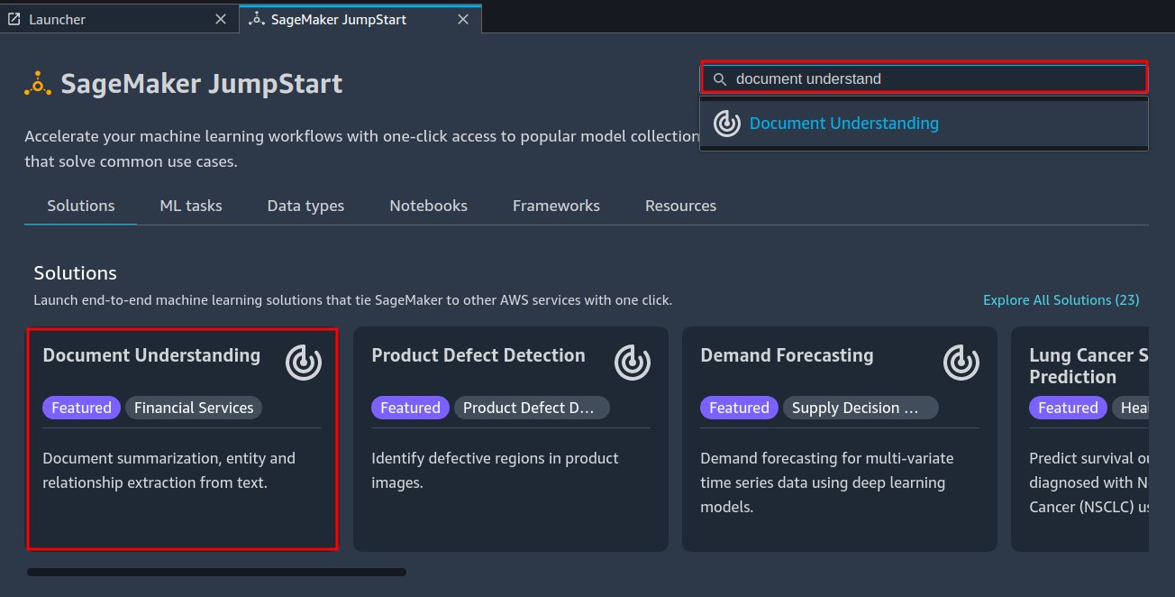
The JumpStart solution templates cover a variety of use cases, under each of which several different solution templates are offered (this Document Understanding solution is under the “Extract and analyze data from documents” use case).
Choose the solution template that best fits your use case from the JumpStart landing page. For more information on specific solutions under each use case and how to launch a JumpStart solution, see Solution Templates.
Solution overview
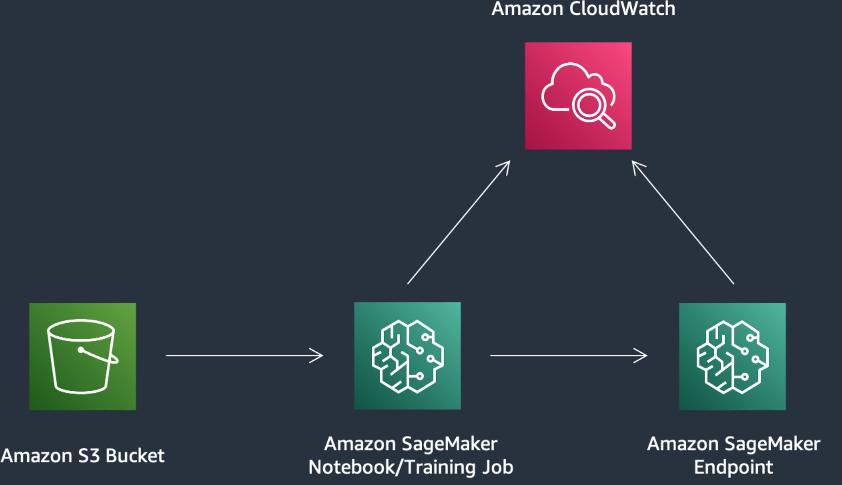
The following image demonstrates how you can use this solution with SageMaker components. The SageMaker training jobs are used to train the various NLP model, and SageMaker endpoints are used to deploy the models in each stage. We use Amazon Simple Storage Service (Amazon S3) alongside SageMaker to store the training data and model artifacts, and Amazon CloudWatch to log training and endpoint outputs.
Open the Document Understanding solution
Navigate to the Document Understanding solution in JumpStart.
Now we can take a closer look at some of the assets that are included in this solution, starting with the demo notebook.
Demo notebook
You can use the demo notebook to send example data to already deployed model endpoints for the document summarization and question answering tasks. The demo notebook quickly allows you to get hands-on experience by querying the example data.
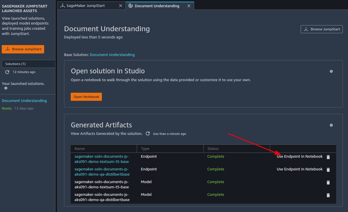
After you launch the Document Understanding solution, open the demo notebook by choosing Use Endpoint in Notebook.
Let’s dive deeper into each of the five main notebooks for this solution.
Prerequisites
In Amazon SageMaker Studio, ensure you’re using the PyTorch 1.10 Python 3.8 CPU Optimized image/kernel to open the notebooks. Training uses five ml.g4dn.2xlarge instances, so you should raise a service limit increase request if your account requires increased limits for this type.
Text classification
Text classification refers to classifying an input sentence to one of the class labels of the training dataset. This notebook demonstrates how to use the JumpStart API for text classification.
Deploy and run inference on the pre-trained model
The text classification model we’ve chosen to use is built upon a text embedding (tensorflow-tc-bert-en-uncased-L-12-H-768-A-12-2) model from TensorFlow Hub, which is pre-trained on Wikipedia and BookCorpus datasets.
The model available for deployment is created by attaching a binary classification layer to the output of the text embedding model, and then fine-tuning the entire model on the SST-2 dataset, which is comprised of positive and negative movie reviews.
To run inference on this model, we first need to download the inference container (deploy_image_uri), inference script (deploy_source_uri), and pre-trained model (base_model_uri). We then pass those as parameters to instantiate a SageMaker model object, which we can then deploy:
model = Model(
    image_uri=deploy_image_uri,
    source_dir=deploy_source_uri,
    model_data=base_model_uri,
    entry_point="inference.py",
    role=aws_role,
    predictor_cls=Predictor,
    name=endpoint_name_tc,
)
# deploy the Model.
base_model_predictor = model.deploy(
    initial_instance_count=1,
    instance_type=inference_instance_type,
    endpoint_name=endpoint_name_tc,
)
After we deploy the model, we assemble some example inputs and query the endpoint:
text1 = "astonishing ... ( frames ) profound ethical and philosophical questions in the form of dazzling pop entertainment"
text2 = "simply stupid , irrelevant and deeply , truly , bottomlessly cynical "
The following code shows our responses:
Inference:
Input text: 'astonishing ... ( frames ) profound ethical and philosophical questions in the form of dazzling pop entertainment'
Model prediction: [0.000452966779, 0.999547064]
Labels: [0, 1]
Predicted Label: 1 # value 0 means negative sentiment and value 1 means positive sentiment

Inference:
Input text: 'simply stupid , irrelevant and deeply , truly , bottomlessly cynical '
Model prediction: [0.998723, 0.00127695734]
Labels: [0, 1]
Predicted Label: 0
Fine-tune the pre-trained model on a custom dataset
We just walked through running inference on a pre-trained BERT model, which was fine-tuned on the SST-2 dataset.
Next, we discuss how to fine-tune a model on a custom dataset with any number of classes. The dataset we use for fine-tuning is still the SST-2 dataset. You can replace this dataset with any dataset that you’re interested in.
We retrieve the training Docker container, training algorithm source, and pre-trained model:
from sagemaker import image_uris, model_uris, script_uris, hyperparameters

model_id, model_version = model_id, "*" # all the other options of model_id are the same as the one in Section 2.
training_instance_type = config.TRAINING_INSTANCE_TYPE

# Retrieve the docker image
train_image_uri = image_uris.retrieve(
    region=None,
    framework=None,
    model_id=model_id,
    model_version=model_version,
    image_scope="training",
    instance_type=training_instance_type,
)
# Retrieve the training script
train_source_uri = script_uris.retrieve(
    model_id=model_id, model_version=model_version, script_scope="training"
)
# Retrieve the pre-trained model tarball to further fine-tune
train_model_uri = model_uris.retrieve(
    model_id=model_id, model_version=model_version, model_scope="training"
)
For algorithm-specific hyperparameters, we start by fetching a Python dictionary of the training hyperparameters that the algorithm accepts with their default values. You can override them with custom values, as shown in the following code:
from sagemaker import hyperparameters

# Retrieve the default hyper-parameters for fine-tuning the model
hyperparameters = hyperparameters.retrieve_default(model_id=model_id, model_version=model_version)

# [Optional] Override default hyperparameters with custom values
hyperparameters["batch-size"] = "64"
hyperparameters["adam-learning-rate"] = "1e-6"
The dataset (SST-2) is split into training, validation, and test sets, where the training set is used to fit the model, the validation set is used to compute evaluation metrics that can be used for HPO, and the test set is used as hold-out data for evaluating model performance. Next, the train and validation dataset are uploaded to Amazon S3 and used to launch the fine-tuning training job:
# Create SageMaker Estimator instance
tc_estimator = Estimator(
    role=role,
    image_uri=train_image_uri,
    source_dir=train_source_uri,
    model_uri=train_model_uri,
    entry_point="transfer_learning.py",
    instance_count=1,
    instance_type=training_instance_type,
    max_run=360000,
    hyperparameters=hyperparameters,
    output_path=s3_output_location,
    tags=[{'Key': config.TAG_KEY, 'Value': config.SOLUTION_PREFIX}],
    base_job_name=training_job_name,
)

training_data_path_updated = f"s3://{config.S3_BUCKET}/{prefix}/train"
# Launch a SageMaker Training job by passing s3 path of the training data
tc_estimator.fit({"training": training_data_path_updated}, logs=True)
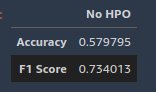
After the fine-tuning job is complete, we deploy the model, run inference on the hold-out test dataset, and compute evaluation metrics. Because it’s a binary classification task, we use the accuracy score and F1 score as the evaluation metrics. A larger value indicates the better performance. The following screenshot shows our results.
Further improve the fine-tuning performance with SageMaker automatic model tuning
In this step, we demonstrate how you can further improve model performance by fine-tuning the model with SageMaker automatic model tuning. Automatic model tuning, also known as hyperparameter optimization (HPO), finds the best version of a model by running multiple training jobs on your dataset with a range of hyperparameters that you specify. It then chooses the hyperparameter values that result in a model that performs the best, as measured by a metric that you choose, on the validation dataset.
First, we set the objective as the accuracy score on the validation data (val_accuracy) and defined metrics for the tuning job by specifying the objective metric name and a regular expression (regex). The regular expression is used to match the algorithm’s log output and capture the numeric values of metrics. Next, we specify hyperparameter ranges to select the best hyperparameter values from. We set the total number of tuning jobs as six and distribute these jobs on three different Amazon Elastic Compute Cloud (Amazon EC2) instances for running parallel tuning jobs. See the following code:
# Define objective metric per framework, based on which the best model will be selected.
metric_definitions_per_model = {
    "tensorflow": {
        "metrics": [{"Name": "val_accuracy", "Regex": "val_accuracy: ([0-9\.]+)"}],
        "type": "Maximize",
    }
}

# You can select from the hyperparameters supported by the model, and configure ranges of values to be searched for training the optimal model.(https://docs.aws.amazon.com/sagemaker/latest/dg/automatic-model-tuning-define-ranges.html)
hyperparameter_ranges = {
    "adam-learning-rate": ContinuousParameter(0.00001, 0.01, scaling_type="Logarithmic")
}

# Increase the total number of training jobs run by AMT, for increased accuracy (and training time).
max_jobs = 6
# Change parallel training jobs run by AMT to reduce total training time, constrained by your account limits.
# if max_jobs=max_parallel_jobs then Bayesian search turns to Random.
max_parallel_jobs = 3
We pass those values to instantiate a SageMaker Estimator object, similar to what we did in the previous fine-tuning step. Instead of calling the fit function of the Estimator object, we pass the Estimator object in as a parameter to the HyperparameterTuner constructor and call the fit function of it to launch tuning jobs:
hp_tuner = HyperparameterTuner(
    tc_estimator,
    metric_definitions["metrics"][0]["Name"],
    hyperparameter_ranges,
    metric_definitions["metrics"],
    max_jobs=max_jobs,
    max_parallel_jobs=max_parallel_jobs,
    objective_type=metric_definitions["type"],
    base_tuning_job_name=tuning_job_name,
)

# Launch a SageMaker Tuning job to search for the best hyperparameters
hp_tuner.fit({"training": training_data_path_updated})
After the tuning jobs are complete, we deploy the model that gives the best evaluation metric score on the validation dataset, perform inference on the same hold-out test dataset we did in the previous section, and compute evaluation metrics.
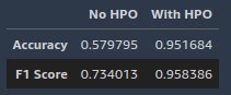
The results show that the model selected by automatic model tuning significantly outperforms the model fine-tuned in the previous section on a hold-out test dataset.
Named entity recognition
Named entity recognition (NER) is the process of detecting and classifying named entities into predefined categories, such as names of persons, organizations, locations, and quantities. There are many real-world use cases for NER, such as recommendation engines, categorizing and assigning customer support tickets to the right department, extracting essential information from patient reports in healthcare, and content classification from news and blogs.
Deploy and run inference on the pre-trained model
We deploy the En_core_web_md model from the spaCy library. spaCy is an open-source NLP library that can be used for various tasks, and has built-in methods for NER. We use an AWS PyTorch Deep Learning Container (DLC) with a script mode and install the spaCy library as a dependency on top of the container.
Next, an entry point for the script (argument entry_point.py) is specified, containing all the code to download and load the En_core_web_md model and perform inference on the data that is sent to the endpoint. Finally, we still need to provide model_data as the pre-trained model for inference. Because the pre-trained En_core_web_md model is downloaded on the fly, which is specified in the entry script, we provide an empty archive file. After the endpoint is deployed, you can invoke the endpoint directly from the notebook using the SageMaker Python SDK’s Predictor. See the following code:
model = PyTorchModel(
    model_data=f"{config.SOURCE_S3_PATH}/artifacts/models/empty.tar.gz",
    entry_point="entry_point.py",
    source_dir="../containers/entity_recognition",
    role=config.IAM_ROLE,
    framework_version="1.5.0",
    py_version="py3",
    code_location="s3://" + config.S3_BUCKET + "/code",
    env={
        "MMS_DEFAULT_RESPONSE_TIMEOUT": "3000"
    }
)
predictor = model.deploy(
    endpoint_name=endpoint_name,
    instance_type=config.HOSTING_INSTANCE_TYPE,
    initial_instance_count=1,
    serializer=JSONSerializer(),
    deserializer=JSONDeserializer()
)
The input data for the model is a textual document. The named entity model extracts noun chunks and named entities in the textual document and classifies them into a number of different types (such as people, places, and organizations). The example input and output are shown in the following code. The start_char parameter indicates the character offset for the start of the span, and end_char indicates the end of the span.
data = {'text': 'Amazon SageMaker is a fully managed service that provides every developer and data scientist with the ability to build, train, and deploy machine learning (ML) models quickly.'}
response = predictor.predict(data=data)

print(response['entities'])
print(response['noun_chunks'])

[{'text': 'Amazon SageMaker', 'start_char': 0, 'end_char': 16, 'label': 'ORG'}]
[{'text': 'Amazon SageMaker', 'start_char': 0, 'end_char': 16}, {'text': 'a fully managed service', 'start_char': 20, 'end_char': 43}, {'text': 'that', 'start_char': 44, 'end_char': 48}, {'text': 'every developer and data scientist', 'start_char': 58, 'end_char': 92}, {'text': 'the ability', 'start_char': 98, 'end_char': 109}, {'text': 'ML', 'start_char': 156, 'end_char': 158}]
Fine-tune the pre-trained model on a custom dataset
In this step, we demonstrate how to fine-tune a pre-trained language models for NER on your own dataset. The fine-tuning step updates the model parameters to capture the characteristic of your own data and improve accuracy. We use the WikiANN (PAN-X) dataset to fine-tune the DistilBERT-base-uncased Transformer model from Hugging Face.
The dataset is split into training, validation, and test sets.
Next, we specify the hyperparameters of the model, and use an AWS Hugging Face DLC with a script mode (argument entry_point) to trigger the fine-tuning job:
hyperparameters = {
    "pretrained-model": "distilbert-base-uncased",
    "learning-rate": 2e-6,
    "num-train-epochs": 2,
    "batch-size": 16,
    "weight-decay": 1e-5,
    "early-stopping-patience": 2,
}

ner_estimator = HuggingFace(
    pytorch_version='1.10.2',
    py_version='py38',
    transformers_version="4.17.0",
    entry_point='training.py',
    source_dir='../containers/entity_recognition/finetuning',
    hyperparameters=hyperparameters,
    role=aws_role,
    instance_count=1,
    instance_type=training_instance_type,
    output_path=f"s3://{bucket}/{prefix}/output",
    code_location=f"s3://{bucket}/{prefix}/output",
    tags=[{'Key': config.TAG_KEY, 'Value': config.SOLUTION_PREFIX}],
    sagemaker_session=sess,
    volume_size=30,
    env={
        'MMS_DEFAULT_RESPONSE_TIMEOUT': '500'
    },
    base_job_name = training_job_name
)
After the fine-tuning job is complete, we deploy an endpoint and query that endpoint with the hold-out test data. To query the endpoint, each text string needs to be tokenized into one or multiple tokens and sent to the transformer model. Each token gets a predicted named entity tag. Because each text string can be tokenized into one or multiple tokens, we need to duplicate the ground truth named entity tag of the string to all the tokens that are associated to it. The notebook provided walks you through the steps to achieve this.
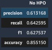
Lastly, we use Hugging Face built-in evaluation metrics seqeval to compute evaluation scores on the hold-out test data. The evaluation metrics used are overall precision, overall recall, overall F1, and accuracy. The following screenshot shows our results.
Further improve the fine-tuning performance with SageMaker automatic model tuning
Similar to text classification, we demonstrate how you can further improve model performance by fine-tuning the model with SageMaker automatic model tuning. To run the tuning job, we need define an objective metric we want to use for evaluating model performance on the validation dataset (F1 score in this case), hyperparameter ranges to select the best hyperparameter values from, as well as tuning job configurations such as maximum number of tuning jobs and number of parallel jobs to launch at a time:
hyperparameters_range = {
    "learning-rate": ContinuousParameter(1e-5, 0.1, scaling_type="Logarithmic"),
    "weight-decay": ContinuousParameter(1e-6, 1e-2, scaling_type="Logarithmic"),
}

tuner = HyperparameterTuner(
    estimator,
    "f1",
    hyperparameters_range,
    [{"Name": "f1", "Regex": "'eval_f1': ([0-9\.]+)"}],
    max_jobs=6,
    max_parallel_jobs=3,
    objective_type="Maximize",
    base_tuning_job_name=tuning_job_name,
)

tuner.fit({
    "train": f"s3://{bucket}/{prefix}/train/",
    "validation": f"s3://{bucket}/{prefix}/validation/",
}, logs=True)
After the tuning jobs are complete, we deploy the model that gives the best evaluation metric score on the validation dataset, perform inference on the same hold-out test dataset we did in the previous section, and compute evaluation metrics.
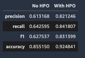
We can see that the model with HPO achieves significantly better performance across all metrics.
Question answering
Question answering is useful when you want to query a large amount of text for specific information. It allows a user to express a question in natural language and get an immediate and brief response. Question answering systems powered by NLP can be used in search engines and phone conversational interfaces.
Deploy and run inference on the pre-trained model
Our pre-trained model is the extractive question answering (EQA) model bert-large-uncased-whole-word-masking-finetuned-squad built on a Transformer model from Hugging Face. We use an AWS PyTorch DLC with a script mode and install the transformers library as a dependency on top of the container. Similar to the NER task, we provide an empty archive file in the argument model_data because the pre-trained model is downloaded on the fly. After the endpoint is deployed, you can invoke the endpoint directly from the notebook using the SageMaker Python SDK’s Predictor. See the following code:
model = PyTorchModel(
    model_data=f"{config.SOURCE_S3_PATH}/artifacts/models/empty.tar.gz",
    entry_point="entry_point.py",
    source_dir="../containers/question_answering",
    role=config.IAM_ROLE,
    framework_version="1.5.0",
    py_version="py3",
    code_location="s3://" + config.S3_BUCKET + "/code",
    env={
        "MODEL_ASSETS_S3_BUCKET": config.SOURCE_S3_BUCKET,
        "MODEL_ASSETS_S3_PREFIX": f"{config.SOURCE_S3_PREFIX}/artifacts/models/question_answering/",
        "MMS_DEFAULT_RESPONSE_TIMEOUT": "3000",
    },
)
After the endpoint is successfully deployed and the predictor is configured, we can try out the question answering model on example inputs. This model has been pretrained on the Stanford Question and Answer Dataset (SQuAD) dataset. This dataset was introduced in the hopes of furthering the field of question answering modeling. It’s a reading comprehension dataset comprised of passages, questions, and answers.
All we need to do is construct a dictionary object with two keys. context is the text that we wish to retrieve information from. question is the natural language query that specifies what information we’re interested in extracting. We call predict on our predictor, and we should get a response from the endpoint that contains the most likely answers:
data = {'question': 'what is my name?', 'context': "my name is thom"}
response = predictor.predict(data=data)
We have the response, and we can print out the most likely answers that have been extracted from the preceding text. Each answer has a confidence score used for ranking (but this score shouldn’t be interpreted as a true probability). In addition to the verbatim answer, you also get the start and end character indexes of the answer from the original context:
print(response['answers'])
[{'score': 0.9793591499328613, 'start': 11, 'end': 15, 'answer': 'thom'},
{'score': 0.02019440196454525, 'start': 0, 'end': 15, 'answer': 'my name is thom'},
{'score': 4.349117443780415e-05, 'start': 3, 'end': 15, 'answer': 'name is thom'}]
Now we fine-tune this model with our own custom dataset to get better results.
Fine-tune the pre-trained model on a custom dataset
In this step, we demonstrate how to fine-tune a pre-trained language models for EQA on your own dataset. The fine-tuning step updates the model parameters to capture the characteristic of your own data and improve accuracy. We use the SQuAD2.0 dataset to fine-tune a text embedding model bert-base-uncased from Hugging Face. The model available for fine-tuning attaches an answer extracting layer to the text embedding model and initializes the layer parameters to random values. The fine-tuning step fine-tunes all the model parameters to minimize prediction error on the input data and returns the fine-tuned model.
Similar to the text classification task, the dataset (SQuAD2.0) is split into training, validation, and test set.
Next, we specify the hyperparameters of the model, and use the JumpStart API to trigger a fine-tuning job:
hyperparameters = {'epochs': '3', 'adam-learning-rate': '2e-05', 'batch-size': '16'}

eqa_estimator = Estimator(
    role=role,
    image_uri=train_image_uri,
    source_dir=train_source_uri,
    model_uri=train_model_uri,
    entry_point="transfer_learning.py",
    instance_count=1,
    instance_type=training_instance_type,
    max_run=360000,
    hyperparameters=hyperparameters,
    output_path=s3_output_location,
    tags=[{'Key': config.TAG_KEY, 'Value': config.SOLUTION_PREFIX}],
    base_job_name=training_job_name,
    debugger_hook_config=False,
)

training_data_path_updated = f"s3://{config.S3_BUCKET}/{prefix}/train"
# Launch a SageMaker Training job by passing s3 path of the training data
eqa_estimator.fit({"training": training_data_path_updated}, logs=True)
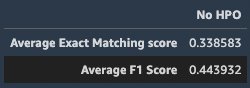
After the fine-tuning job is complete, we deploy the model, run inference on the hold-out test dataset, and compute evaluation metrics. The evaluation metrics used are the average exact matching score and average F1 score. The following screenshot shows the results.
Further improve the fine-tuning performance with SageMaker automatic model tuning
Similar to the previous sections, we use a HyperparameterTuner object to launch tuning jobs:
hyperparameter_ranges = {
    "adam-learning-rate": ContinuousParameter(0.00001, 0.01, scaling_type="Logarithmic"),
    "epochs": IntegerParameter(3, 10),
    "train-only-top-layer": CategoricalParameter(["True", "False"]),
}

hp_tuner = HyperparameterTuner(
    eqa_estimator,
    metric_definitions["metrics"][0]["Name"],
    hyperparameter_ranges,
    metric_definitions["metrics"],
    max_jobs=max_jobs,
    max_parallel_jobs=max_parallel_jobs,
    objective_type=metric_definitions["type"],
    base_tuning_job_name=training_job_name,
)

# Launch a SageMaker Tuning job to search for the best hyperparameters
hp_tuner.fit({"training": training_data_path_updated})
After the tuning jobs are complete, we deploy the model that gives the best evaluation metric score on the validation dataset, perform inference on the same hold-out test dataset we did in the previous section, and compute evaluation metrics.
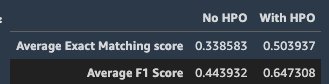
We can see that the model with HPO shows a significantly better performance on the hold-out test data.
Relationship extraction
Relationship extraction is the task of extracting semantic relationships from text, which usually occur between two or more entities. Relationship extraction plays an important role in extracting structured information from unstructured sources such as raw text. In this notebook, we demonstrate two use cases of relationship extraction.
Fine-tune the pre-trained model on a custom dataset
We use a relationship extraction model built on a BERT-base-uncased model using transformers from the Hugging Face transformers library. The model for fine-tuning attaches a linear classification layer that takes a pair of token embeddings outputted by the text embedding model and initializes the layer parameters to random values. The fine-tuning step fine-tunes all the model parameters to minimize prediction error on the input data and returns the fine-tuned model.
The dataset we fine-tune the model is SemEval-2010 Task 8. The model returned by fine-tuning can be further deployed for inference.
The dataset contains training, validation, and test sets.
We use the AWS PyTorch DLC with a script mode from the SageMaker Python SDK, where the transformers library is installed as the dependency on top of the container. We define the SageMaker PyTorch estimator and a set of hyperparameters such as the pre-trained model, learning rate, and epoch numbers to perform the fine-tuning. The code for fine-tuning the relationship extraction model is defined in the entry_point.py. See the following code:
hyperparameters = {
    "pretrained-model": "bert-base-uncased",
    "learning-rate": 0.0002,
    "max-epoch": 2,
    "weight-decay": 0,
    "batch-size": 16,
    "accumulate-grad-batches": 2,
    "gradient-clip-val": 1.0
}

re_estimator = PyTorch(
    framework_version='1.5.0',
    py_version='py3',
    entry_point='entry_point.py',
    source_dir='../containers/relationship_extraction',
    hyperparameters=hyperparameters,
    role=aws_role,
    instance_count=1,
    instance_type=train_instance_type,
    output_path=f"s3://{bucket}/{prefix}/output",
    code_location=f"s3://{bucket}/{prefix}/output",
    base_job_name=training_job_name,
    tags=[{'Key': config.TAG_KEY, 'Value': config.SOLUTION_PREFIX}],
    sagemaker_session=sess,
    volume_size=30,
    env={
        'MMS_DEFAULT_RESPONSE_TIMEOUT': '500'
    },
    debugger_hook_config=False
)

re_estimator.fit(
    {
        "train": f"s3://{bucket}/{prefix}/train/",
        "validation": f"s3://{bucket}/{prefix}/validation/",
    }
)
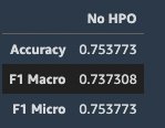
The training job takes approximately 31 minutes to complete. We use this model to perform inference on the hold-out test set and evaluate the results using accuracy, F1 macro, and F1 micro scores. The following screenshot shows the evaluation scores.
Further improve the fine-tuning performance with SageMaker automatic model tuning
Similar to the previous sections, we use a HyperparameterTuner object to interact with SageMaker hyperparameter tuning APIs. We can start the hyperparameter tuning job by calling the fit method:
hyperparameters = {
    "max-epoch": 2,
    "weight-decay": 0,
    "batch-size": 16,
    "accumulate-grad-batches": 2,
    "gradient-clip-val": 1.0
}

estimator = PyTorch(
    framework_version='1.5.0',
    py_version='py3',
    entry_point='entry_point.py',
    source_dir='../containers/relationship_extraction',
    hyperparameters=hyperparameters,
    role=aws_role,
    instance_count=1,
    instance_type=train_instance_type,
    output_path=f"s3://{bucket}/{prefix}/output",
    code_location=f"s3://{bucket}/{prefix}/output",
    base_job_name=tuning_job_name,
    tags=[{'Key': config.TAG_KEY, 'Value': config.SOLUTION_PREFIX}],
    sagemaker_session=sess,
    volume_size=30,
    env={
        'MMS_DEFAULT_RESPONSE_TIMEOUT': '500'
    },
    debugger_hook_config=False

    re_tuner = HyperparameterTuner(
    estimator,
    metric_definitions["metrics"][0]["Name"],
    hyperparameter_ranges,
    metric_definitions["metrics"],
    max_jobs=max_jobs,
    max_parallel_jobs=max_parallel_jobs,
    objective_type=metric_definitions["type"],
    base_tuning_job_name=tuning_job_name,
)

re_tuner.fit({
    "train": f"s3://{bucket}/{prefix}/train/",
    "validation": f"s3://{bucket}/{prefix}/validation/",
})
When the hyperparameter tuning job is complete, we perform inference and check the evaluation score.
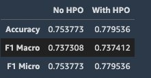
We can see that the model with HPO shows better performance on the hold-out test data.
Document summarization
Document or text summarization is the task of condensing large amounts of text data into a smaller subset of meaningful sentences that represent the most important or relevant information within the original content. Document summarization is a useful technique to distill important information from large amounts of text data to a few sentences. Text summarization is used in many use cases, such as document processing and extracting information from blogs, articles, and news.
This notebook demonstrates deploying the document summarization model T5-base from the Hugging Face transformers library. We also test the deployed endpoints using a text article and evaluate results using the Hugging Face built-in evaluation metric ROUGE.
Similar to the question answering and NER notebooks, we use the PyTorchModel from the SageMaker Python SDK along with an entry_point.py script to load the T5-base model to an HTTPS endpoint. After the endpoint is successfully deployed, we can send a text article to the endpoint to get a prediction response:
ARTICLE = """ Documents are a primary tool for communication,
collaboration, record keeping, and transactions across industries,
including financial, medical, legal, and real estate. The format of data
can pose an extra challenge in data extraction, especially if the content
is typed, handwritten, or embedded in a form or table. Furthermore,
extracting data from your documents is manual, error-prone, time-consuming,
expensive, and does not scale. Amazon Textract is a machine learning (ML)
service that extracts printed text and other data from documents as well as
tables and forms. We’re pleased to announce two new features for Amazon
Textract: support for handwriting in English documents, and expanding
language support for extracting printed text from documents typed in
Spanish, Portuguese, French, German, and Italian. Many documents, such as
medical intake forms or employment applications, contain both handwritten
and printed text. The ability to extract text and handwriting has been a
need our customers have asked us for. Amazon Textract can now extract
printed text and handwriting from documents written in English with high
confidence scores, whether it’s free-form text or text embedded in tables
and forms. Documents can also contain a mix of typed text or handwritten
text. The following image shows an example input document containing a mix
of typed and handwritten text, and its converted output document.."""

data = {'text': ARTICLE}
response = predictor.predict(data=data)
print(response['summary'])

"""Amazon Textract is a machine learning (ML) service that extracts printed text
and other data from documents as well as tables and forms .
customers can now extract and process documents in more languages .
support for handwriting in english documents and expanding language support for extracting
printed text ."""
Next, we evaluate and compare the text article and summarization result using the the ROUGE metric. Three evaluation metrics are calculated: rougeN, rougeL, and rougeLsum. rougeN measures the number of matching n-grams between the model-generated text (summarization result) and a reference (input text). The metrics rougeL and rougeLsum measure the longest matching sequences of words by looking for the longest common substrings in the generated and reference summaries. For each metric, confidence intervals for precision, recall, and F1 score are calculated.See the following code:
results = rouge.compute(predictions=[response['summary']], references=[ARTICLE])

rouge1: AggregateScore(low=Score(precision=1.0, recall=0.1070615034168565, fmeasure=0.1934156378600823),
mid=Score(precision=1.0, recall=0.1070615034168565, fmeasure=0.1934156378600823), high=Score(precision=1.0, recall=0.1070615034168565, fmeasure=0.1934156378600823))

rouge2: AggregateScore(low=Score(precision=0.9565217391304348, recall=0.1004566210045662, fmeasure=0.18181818181818182),
mid=Score(precision=0.9565217391304348, recall=0.1004566210045662, fmeasure=0.18181818181818182), high=Score(precision=0.9565217391304348, recall=0.1004566210045662,
fmeasure=0.18181818181818182))

rougeL: AggregateScore(low=Score(precision=0.8085106382978723, recall=0.08656036446469248, fmeasure=0.15637860082304528),
mid=Score(precision=0.8085106382978723, recall=0.08656036446469248, fmeasure=0.15637860082304528), high=Score(precision=0.8085106382978723, recall=0.08656036446469248,
fmeasure=0.15637860082304528))

rougeLsum: AggregateScore(low=Score(precision=0.9787234042553191, recall=0.10478359908883828, fmeasure=0.18930041152263374),
mid=Score(precision=0.9787234042553191, recall=0.10478359908883828, fmeasure=0.18930041152263374), high=Score(precision=0.9787234042553191, recall=0.10478359908883828,
fmeasure=0.18930041152263374))
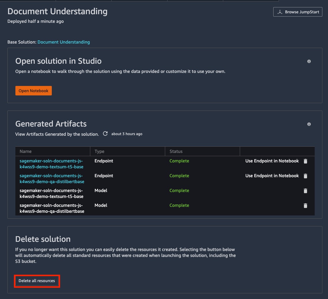
Clean up
Resources created for this solution can be deleted using the Delete all resources button from the SageMaker Studio IDE. Each notebook also provides a clean-up section with the code to delete the endpoints.
Conclusion
In this post, we demonstrated how to utilize state-of-the-art ML techniques to solve five different NLP tasks: document summarization, text classification, question and answering, named entity recognition, and relationship extraction using Jumpstart. Get started with Jumpstart now!
About the Authors
 Dr. Xin Huang is an Applied Scientist for Amazon SageMaker JumpStart and Amazon SageMaker built-in algorithms. He focuses on developing scalable machine learning algorithms. His research interests are in the area of natural language processing, explainable deep learning on tabular data, and robust analysis of non-parametric space-time clustering. He has published many papers in ACL, ICDM, KDD conferences, and Royal Statistical Society: Series A journal.
 Vivek Gangasani is a Senior Machine Learning Solutions Architect at Amazon Web Services. He helps Startups build and operationalize AI/ML applications. He is currently focused on combining his background in Containers and Machine Learning to deliver solutions on MLOps, ML Inference and low-code ML. In his spare time, he enjoys trying new restaurants and exploring emerging trends in AI and deep learning.
 Geremy Cohen is a Solutions Architect with AWS where he helps customers build cutting-edge, cloud-based solutions. In his spare time, he enjoys short walks on the beach, exploring the bay area with his family, fixing things around the house, breaking things around the house, and BBQing.
 Neelam Koshiya is an enterprise solution architect at AWS. Her current focus is to help enterprise customers with their cloud adoption journey for strategic business outcomes. In her spare time, she enjoys reading and being outdoors.
Read More


 Brandon Nair is a Senior Product Manager for Amazon Forecast. His professional interest lies in creating scalable machine learning services and applications. Outside of work he can be found exploring national parks, perfecting his golf swing or planning an adventure trip.
 Manas Dadarkar is a Software Development Manager owning the engineering of the Amazon Forecast service. He is passionate about the applications of machine learning and making ML technologies easily available for everyone to adopt and deploy to production. Outside of work, he has multiple interests including travelling, reading and spending time with friends and family.
 Bharat Nandamuri is a Sr Software Engineer working on Amazon Forecast. He is passionate about building high scale backend services with focus on Engineering for ML systems. Outside of work, he enjoys playing chess, hiking and watching movies.
 Gaurav Gupta is an Applied Scientist at AWS AI labs and Amazon Forecast. His research interests lie in machine learning for sequential data, operator learning for partial differential equations, wavelets. He completed his PhD from University of Southern California before joining AWS.