The National Football League (NFL) is one of the most popular sports leagues in the United States and is the most valuable sports league in the world. The NFL, BioCore, and AWS are committed to advancing human understanding around the diagnosis, prevention, and treatment of sports-related injuries to make the game of football safer. More information regarding the NFL Player Health and Safety efforts is available on the NFL website.
The AWS Professional Services team has partnered with the NFL and Biocore to provide machine learning (ML)-based solutions for identifying helmet impacts from game footage using computer vision (CV) techniques. With multiple camera views available from each game, we have developed solutions to identify helmet impacts from each of these views and merge the helmet impact results.
The motivation behind utilizing multiple camera views comes from the limitation of information when the impact events are captured with only one view. With only one perspective, some players might occlude each other or be blocked by other objects on the field. Therefore, adding more perspectives allows our ML system to identify more impacts that aren’t visible in a single view. To showcase the results of our fusion process and how the team uses visualization tools to help evaluate the model performance, we have developed a codebase to visually overlay the multiple view detection results. This process helps identify the actual number of impacts individual players experience by removing duplicate impacts detected in multiple views.
In this post, we use the publicly available dataset from the NFL – Impact Detection Kaggle competition and show results for merging two views. The dataset includes helmet bounding boxes at every frame and impact labels found in each video. In particular, we focus on deduplicating and visualizing videos with the ID 57583_000082 in endzone and sideline views. You can download the endzone and sideline videos, and also the ground truth labels.
Prerequisites
The solution requires the following:
Get started on SageMaker Studio Lab and install the required packages
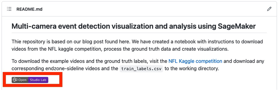
You can run the notebook from the GitHub repository or from SageMaker Studio Lab. In this post, we run the notebook from a SageMaker Studio Lab environment. We are choosing SageMaker Studio Lab because it is free, provides powerful CPU and GPU user sessions, and 15GB of persistent storage that will automatically save your environment, enabling you to pick up where you left off. To use SageMaker Studio Lab, request and set up a new account. After the account is approved, complete the following steps:
- Visit the aws-samples GitHub repo.
- In the
README section, choose Open Studio Lab.
This redirects you to your SageMaker Studio Lab environment.
- Select your CPU compute type, then choose Start Runtime.
- After the runtime starts, choose Copy to Project, which opens a new window with the Jupyter Lab environment.
Now you’re ready to use the notebook!
- Open
fuse_and_visualize_multiview_impacts.ipynb and follow the instructions in the notebook.
The first cell in the notebook installs the necessary Python packages such as pandas and OpenCV:
%pip install pandas
%pip install opencv-contrib-python-headless
Import all the necessary Python packages and set pandas options for better visualization experience:
import os
import cv2
import pandas as pd
import numpy as np
pd.set_option('mode.chained_assignment', None)
We use pandas for ingesting and parsing through the CSV file with the annotated helmet bounding boxes as well as impacts. We use NumPy mainly for manipulating arrays and matrices. We use OpenCV for reading, writing, and manipulating image data in Python.
Prepare the data by fusing results from two views
To fuse the two perspectives together, we use the train_labels.csv from the Kaggle competition as an example because it contains ground truth impacts from both the endzone and sideline. The following function takes the input dataset and outputs a fused dataframe that is deduplicated for all the plays in the input dataset:
def prep_data(df):
    df['game_play'] = df['gameKey'].astype('str') + '_' + df['playID'].astype('str').str.zfill(6)
    return df

def dedup_view(df, windows):
    # define view
    df = df.sort_values(by='frame')
    view_columns = ['frame', 'left', 'width', 'top', 'height', 'video']
    common_columns = ['game_play', 'label', 'view', 'impactType']
    label_cleaned = df[view_columns + common_columns]

    # rename columns
    sideline_column_rename = {col: 'Sideline_' + col for col in view_columns}
    endzone_column_rename = {col: 'Endzone_' + col for col in view_columns}
    sideline_columns = list(sideline_column_rename.values())

    # create two dataframes, one for sideline, one for endzone
    label_endzone = label_cleaned.query('view == "Endzone"')
    label_endzone.rename(columns=endzone_column_rename, inplace=True)
    label_sideline = label_cleaned.query('view == "Sideline"')
    label_sideline.rename(columns=sideline_column_rename, inplace=True)

    # prepare sideline labels
    label_sideline['is_dup'] = False
    for columns in sideline_columns:
        label_endzone[columns] = np.nan
    label_endzone['is_dup'] = False

    # iterrate endzone rows to find matches and dedup
    for index, row in label_endzone.iterrows():
        player = row['label']
        frame = row['Endzone_frame']
        impact_type = row['impactType']
        sideline_row = label_sideline[(label_sideline['label'] == player) &
                                      ((label_sideline['Sideline_frame'] >= frame - windows // 2) &
                                       (label_sideline['Sideline_frame'] <= frame + windows // 2 + 1)) &
                                      (label_sideline['is_dup'] == False) &
                                      (label_sideline['impactType'] == impact_type)]

        if len(sideline_row) > 0:
            sideline_index = sideline_row.index[0]
            label_sideline['is_dup'].loc[sideline_index] = True

            for col in sideline_columns:
                label_endzone[col].loc[index] = sideline_row.iloc[0][col]
            label_endzone['is_dup'].loc[index] = True

    # calculate overlap perc
    not_dup_sideline = label_sideline[label_sideline['is_dup'] == False]
    final_output = pd.concat([not_dup_sideline, label_endzone])
    return final_output

def fuse_df(raw_df, windows):
    outputs = []
    all_game_play = raw_df['game_play'].unique()
    for game_play in all_game_play:
        df = raw_df.query('game_play ==@game_play')
        output = dedup_view(df, windows)
        outputs.append(output)

    output_df = pd.concat(outputs)
    output_df['gameKey'] = output_df['game_play'].apply(lambda x: x.split('_')[0]).map(int)
    output_df['playID'] = output_df['game_play'].apply(lambda x: x.split('_')[1]).map(int)
    return output_df
To run the function, we run the following code block to provide the location of the train_labels.csv data and then perform data preparation to add an additional column and extract only the impact rows. After running the function, we save the output to a dataframe variable called fused_df.
# read the annotated impact data from train_labels.csv
ground_truth = pd.read_csv('train_labels.csv')

# prepare game_play column using pipe(prep_data) function in pandas then filter the dataframe for just rows with impacts
ground_truth = ground_truth.pipe(prep_data).query('impact == 1')

# loop over all the unique game_plays and deduplicate the impact results from sideline and endzone
fused_df = fuse_df(ground_truth, windows=30)
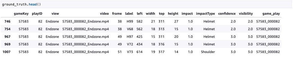
The following screenshot shows the ground truth.
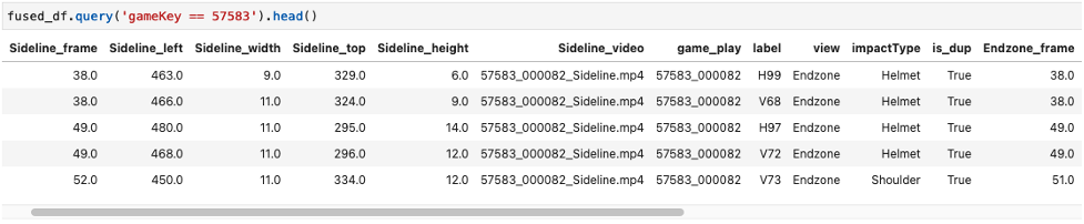
The following screenshot shows the fused dataframe examples.
Graph and video code
After we fuse the impact results, we use the generated fused_df to overlay the results onto our endzone and sideline videos and merge the two views together. We use the following function for this, and the inputs needed are the paths to the endzone video, sideline video, fused_df dataframe, and the final output path for the newly generated video. The functions used in this section are described in the markdown section of the notebook used in SageMaker Studio Lab.
def get_video_and_metadata(vid_path):
    vid = cv2.VideoCapture(vid_path)
    total_frame_number = vid.get(cv2.CAP_PROP_FRAME_COUNT)
    width = int(vid.get(cv2.CAP_PROP_FRAME_WIDTH))
    height = int(vid.get(cv2.CAP_PROP_FRAME_HEIGHT))
    fps = vid.get(cv2.CAP_PROP_FPS)
    return vid, total_frame_number, width, height, fps

def overlay_impacts(frame, fused_df, game_key, play_id, frame_cnt, h1):
    # look for duplicates
    duplicates = fused_df.query(f"gameKey == {int(game_key)} and
                                  playID == {int(play_id)} and
                                  is_dup == True and
                                  Sideline_frame == @frame_cnt")

    frame_has_impact = False

    if len(duplicates) > 0:
        for duplicate in duplicates.itertuples(index=False):
            if frame_cnt == duplicate.Sideline_frame:
                frame_has_impact = True

            if frame_has_impact:
                cv2.rectangle(frame, #frame to be edited
                              (int(duplicate.Sideline_left), int(duplicate.Sideline_top)), #(x,y) of top left corner
                              (int(duplicate.Sideline_left) + int(duplicate.Sideline_width), int(duplicate.Sideline_top) + int(duplicate.Sideline_height)), #(x,y) of bottom right corner
                              (0,0,255), #RED boxes
                              thickness=3)

                cv2.rectangle(frame, #frame to be edited
                              (int(duplicate.Endzone_left), int(duplicate.Endzone_top)+ h1), #(x,y) of top left corner
                              (int(duplicate.Endzone_left) + int(duplicate.Endzone_width), int(duplicate.Endzone_top) + int(duplicate.Endzone_height) + h1), #(x,y) of bottom right corner
                              (0,0,255), #RED boxes
                              thickness=3)

                cv2.line(frame, #frame to be edited
                         (int(duplicate.Sideline_left), int(duplicate.Sideline_top)), #(x,y) of point 1 in a line
                         (int(duplicate.Endzone_left), int(duplicate.Endzone_top) + h1), #(x,y) of point 2 in a line
                         (255, 255, 255), # WHITE lines
                         thickness=4)

            else:
                # if no duplicates, look for sideline then endzone and add to the view
                sl_impacts = fused_df.query(f"gameKey == {int(game_key)} and
                                              playID == {int(play_id)} and
                                              is_dup == False and
                                              view == 'Sideline' and
                                              Sideline_frame == @frame_cnt")

                if len(sl_impacts) > 0:
                    for impact in sl_impacts.itertuples(index=False):
                        if frame_cnt == impact.Sideline_frame:
                            frame_has_impact = True

                        if frame_has_impact:
                            cv2.rectangle(frame, #frame to be edited
                                          (int(impact.Sideline_left), int(impact.Sideline_top)), #(x,y) of top left corner
                                          (int(impact.Sideline_left) + int(impact.Sideline_width), int(impact.Sideline_top) + int(impact.Sideline_height)), #(x,y) of bottom right corner
                                          (0, 255, 255), #YELLOW BOXES
                                          thickness=3)

                ez_impacts = fused_df.query(f"gameKey == {int(game_key)} and
                                              playID == {int(play_id)} and
                                              is_dup == False and
                                              view == 'Endzone' and
                                              Endzone_frame == @frame_cnt")

                if len(ez_impacts) > 0:
                    for impact in ez_impacts.itertuples(index=False):
                        if frame_cnt == impact.Endzone_frame:
                            frame_has_impact = True

                        if frame_has_impact:
                            cv2.rectangle(frame, #frame to be edited
                                          (int(impact.Endzone_left), int(impact.Endzone_top)+ h1), #(x,y) of top left corner
                                          (int(impact.Endzone_left) + int(impact.Endzone_width), int(impact.Endzone_top) + int(impact.Endzone_height) + h1 ), #(x,y) of bottom right corner
                                          (0, 255, 255), #YELLOW BOXES
                                          thickness=3)

    return frame, frame_has_impact

def generate_impact_video(ez_vid_path:str,
                          sl_vid_path:str,
                          fused_df:pd.DataFrame,
                          output_path:str,
                          freeze_impacts=True):

    #define video codec to be used for
    VIDEO_CODEC = "MP4V"

    # parse game_key and play_id information from the name of the files
    game_key = os.path.basename(ez_vid_path).split('_')[0] # parse game_key
    play_id = os.path.basename(ez_vid_path).split('_')[1] # parse play_id

    # get metadata such as total frame number, width, height and frames per second (FPS) from endzone (ez) and sideline (sl) videos
    ez_vid, ez_total_frame_number, ez_width, ez_height, ez_fps = get_video_and_metadata(ez_vid_path)
    sl_vid, sl_total_frame_number, sl_width, sl_height, sl_fps = get_video_and_metadata(sl_vid_path)

    # define a video writer for the output video
    output_video = cv2.VideoWriter(output_path, #output file name
                                   cv2.VideoWriter_fourcc(*VIDEO_CODEC), #Video codec
                                   ez_fps, #frames per second in the output video
                                  (ez_width, ez_height+sl_height)) # frame size with stacking video vertically

    # find shorter video and use the total frame number from the shorter video for the output video
    total_frame_number = int(min(ez_total_frame_number, sl_total_frame_number))

    # iterate through each frame from endzone and sideline
    for frame_cnt in range(total_frame_number):
        frame_has_impact = False
        frame_near_impact = False

        # reading frames from both endzone and sideline
        ez_ret, ez_frame = ez_vid.read()
        sl_ret, sl_frame = sl_vid.read()

        # creating strings to be added to the output frames
        img_name = f"Game key: {game_key}, Play ID: {play_id}, Frame: {frame_cnt}"
        video_frame = f'{game_key}_{play_id}_{frame_cnt}'

        if ez_ret == True and sl_ret == True:
            h, w, c = ez_frame.shape
            h1,w1,c1 = sl_frame.shape

            if h != h1 or w != w1: # resize images if they're different
                ez_frame = cv2.resize(ez_frame,(w1,h1))

            frame = np.concatenate((sl_frame, ez_frame), axis=0) # stack the frames vertically

            frame, frame_has_impact = overlay_impacts(frame, fused_df, game_key, play_id, frame_cnt, h1)

            cv2.putText(frame, #image frame to be modified
                        img_name, #string to be inserted
                        (30, 30), #(x,y) location of the string
                        cv2.FONT_HERSHEY_SIMPLEX, #font
                        1, #scale
                        (255, 255, 255), #WHITE letters
                        thickness=2)

            cv2.putText(frame, #image frame to be modified
                        str(frame_cnt), #frame count string to be inserted
                        (w1-75, h1-20), #(x,y) location of the string in the top view
                        cv2.FONT_HERSHEY_SIMPLEX, #font
                        1, #scale
                        (255, 255, 255), # WHITE letters
                        thickness=2)

            cv2.putText(frame, #image frame to be modified
                        str(frame_cnt), #frame count string to be inserted
                        (w1-75, h1+h-20), #(x,y) location of the string in the bottom view
                        cv2.FONT_HERSHEY_SIMPLEX, #font
                        1, #scale
                        (255, 255, 255), # WHITE letters
                        thickness=2)

            output_video.write(frame)

            # Freeze for 60 frames on impacts
            if frame_has_impact and freeze_impacts:
                for _ in range(60):
                    output_video.write(frame)
        else:
            break

        frame_cnt += 1

    output_video.release()
    return
To run these functions, we can provide an input as shown in the following code, which generates a video called output.mp4:
generate_impact_video('57583_000082_Endzone.mp4',
                      '57583_000082_Sideline.mp4',
                      fused_df,
                      'output.mp4')
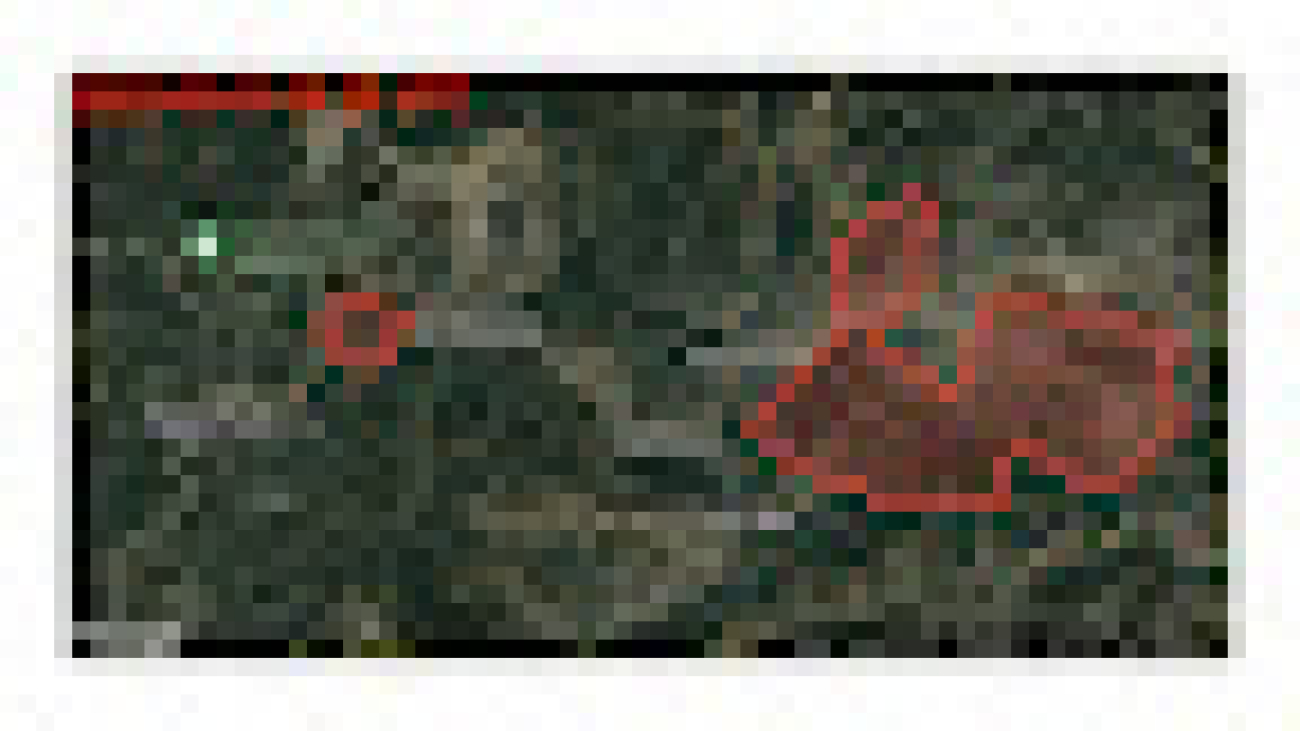
This generates a video as shown in the following example, where the red bounding boxes are impacts found in both endzone and sideline views, and the yellow bounding boxes are impacts that are found in just one view in either the endzone or sideline.
Conclusion
In this post, we demonstrated how the NFL, Biocore, and the AWS ProServe teams are working together to improve impact detection by fusing results from multiple views. This allows the teams to debug and visualize how the model is performing qualitatively. This process can easily be scaled up to three or more views; in our projects, we have utilized up to seven different views. Detecting helmet impacts by watching videos from only one view can be difficult due to view obstruction, but detecting impacts from multiple views and fusing the results allows us to improve our model performance.
To experiment with this solution, visit the aws-samples GitHub repo and refer to the fuse_and_visualize_multiview_impacts.ipynb notebook. Similar techniques can also be applied to other industries such as manufacturing, retail, and security, where having multiple views would benefit the ML system to better identify targets with a more comprehensive view.
For more information regarding NFL Player Health and Safety, visit the NFL website and NFL Explained: Innovation in Player Health & Safety.
About the authors
 Chris Boomhower is a Machine Learning Engineer at AWS Professional Services. Chris has over 6 years experience developing supervised and unsupervised Machine Learning solutions across various industries. Today, he spends most his time helping customers in sports, healthcare, and agriculture industries design and build scalable, end-to-end, Machine Learning solutions.
 Ben Fenker is a Senior Data Scientist in AWS Professional Services and has helped customers build and deploy ML solutions in industries ranging from sports to healthcare to manufacturing. He has a Ph.D. in physics from Texas A&M University and 6 years of industry experience. Ben enjoys baseball, reading, and raising his kids.
 Sam Huddleston is a Principal Data Scientist at Biocore LLC, who serves as the Technology Lead for the NFL’s Digital Athlete program. Biocore is a team of world-class engineers based in Charlottesville, Virginia, that provides research, testing, biomechanics expertise, modeling and other engineering services to clients dedicated to the understanding and reduction of injury.
 Jarvis Lee is a Senior Data Scientist with AWS Professional Services. He has been with AWS for over five years, working with customers on machine learning and computer vision problems. Outside of work, he enjoys riding bicycles.
 Tyler Mullenbach is the Global Practice Lead for ML with AWS Professional Services. He is responsible for driving the strategic direction of ML for Professional Services and ensuring that customers realize transformative business achievements through the adoption of ML technologies.
 Kevin Song is a Data Scientist at AWS Professional Services. He holds a PhD in Biophysics and has over 5 years of industry experience in building computer vision and machine learning solutions.
 Betty Zhang is a data scientist with 10 years of experience in data and technology. Her passion is to build innovative machine learning solutions to drive transformational changes for companies. In her spare time, she enjoys traveling, reading and learning about new technologies.
Read More


 Tesfagabir Meharizghi is a Data Scientist at the

 Kyeong Hoon (Jonathan) Jung is a senior software engineer at the National Football League. He has been with the Next Gen Stats team for the last seven years helping to build out the platform from streaming the raw data, building out microservices to process the data, to building API’s that exposes the processed data. He has collaborated with the Amazon Machine Learning Solutions Lab in providing clean data for them to work with as well as providing domain knowledge about the data itself. Outside of work, he enjoys cycling in Los Angeles and hiking in the Sierras.
 Michael Chi is a Senior Director of Technology overseeing Next Gen Stats and Data Engineering at the National Football League. He has a degree in Mathematics and Computer Science from the University of Illinois at Urbana Champaign. Michael first joined the NFL in 2007 and has primarily focused on technology and platforms for football statistics. In his spare time, he enjoys spending time with his family outdoors.
 Mike Band is a Senior Manager of Research and Analytics for Next Gen Stats at the National Football League. Since joining the team in 2018, he has been responsible for ideation, development, and communication of key stats and insights derived from player-tracking data for fans, NFL broadcast partners, and the 32 clubs alike. Mike brings a wealth of knowledge and experience to the team with a master’s degree in analytics from the University of Chicago, a bachelor’s degree in sport management from the University of Florida, and experience in both the scouting department of the Minnesota Vikings and the recruiting department of Florida Gator Football.
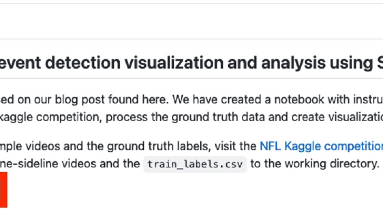


 NVIDIA GeForce NOW (@NVIDIAGFN)