Multilingual Machine Translation promises to improve translation quality between non-English languages. This is advantageous for several reasons, namely lower latency (no need to translate twice), and reduced error cascades (e.g. , avoiding losing gender and formality information when translating through English). On the downside, adding more languages reduces model capacity per language, which is usually countered by increasing the overall model size, making training harder and inference slower. In this work, we introduce Language-Specific Transformer Layers (LSLs), which allow us to increase…Apple Machine Learning Research
PointConvFormer: Revenge of the Point-based Convolution
We introduce PointConvFormer, a novel building block for point cloud based deep network architectures. Inspired by generalization theory, PointConvFormer combines ideas from point convolution, where filter weights are only based on relative position, and Transformers which utilize feature-based attention. In PointConvFormer, attention computed from feature difference between points in the neighborhood is used to modify the convolutional weights at each point. Hence, we preserved the invariances from point convolution, whereas attention helps to select relevant points in the neighborhood for…Apple Machine Learning Research

F-VLM: Open-vocabulary object detection upon frozen vision and language models
Detection is a fundamental vision task that aims to localize and recognize objects in an image. However, the data collection process of manually annotating bounding boxes or instance masks is tedious and costly, which limits the modern detection vocabulary size to roughly 1,000 object classes. This is orders of magnitude smaller than the vocabulary people use to describe the visual world and leaves out many categories. Recent vision and language models (VLMs), such as CLIP, have demonstrated improved open-vocabulary visual recognition capabilities through learning from Internet-scale image-text pairs. These VLMs are applied to zero-shot classification using frozen model weights without the need for fine-tuning, which stands in stark contrast to the existing paradigms used for retraining or fine-tuning VLMs for open-vocabulary detection tasks.
Intuitively, to align the image content with the text description during training, VLMs may learn region-sensitive and discriminative features that are transferable to object detection. Surprisingly, features of a frozen VLM contain rich information that are both region sensitive for describing object shapes (second column below) and discriminative for region classification (third column below). In fact, feature grouping can nicely delineate object boundaries without any supervision. This motivates us to explore the use of frozen VLMs for open-vocabulary object detection with the goal to expand detection beyond the limited set of annotated categories.
 |
| We explore the potential of frozen vision and language features for open-vocabulary detection. The K-Means feature grouping reveals rich semantic and region-sensitive information where object boundaries are nicely delineated (column 2). The same frozen features can classify groundtruth (GT) regions well without fine-tuning (column 3). |
In “F-VLM: Open-Vocabulary Object Detection upon Frozen Vision and Language Models”, presented at ICLR 2023, we introduce a simple and scalable open-vocabulary detection approach built upon frozen VLMs. F-VLM reduces the training complexity of an open-vocabulary detector to below that of a standard detector, obviating the need for knowledge distillation, detection-tailored pre-training, or weakly supervised learning. We demonstrate that by preserving the knowledge of pre-trained VLMs completely, F-VLM maintains a similar philosophy to ViTDet and decouples detector-specific learning from the more task-agnostic vision knowledge in the detector backbone. We are also releasing the F-VLM code along with a demo on our project page.
Learning upon frozen vision and language models
We desire to retain the knowledge of pretrained VLMs as much as possible with a view to minimize effort and cost needed to adapt them for open-vocabulary detection. We use a frozen VLM image encoder as the detector backbone and a text encoder for caching the detection text embeddings of offline dataset vocabulary. We take this VLM backbone and attach a detector head, which predicts object regions for localization and outputs detection scores that indicate the probability of a detected box being of a certain category. The detection scores are the cosine similarity of region features (a set of bounding boxes that the detector head outputs) and category text embeddings. The category text embeddings are obtained by feeding the category names through the text model of pretrained VLM (which has both image and text models)r.
The VLM image encoder consists of two parts: 1) a feature extractor and 2) a feature pooling layer. We adopt the feature extractor for detector head training, which is the only step we train (on standard detection data), to allow us to directly use frozen weights, inheriting rich semantic knowledge (e.g., long-tailed categories like martini, fedora hat, pennant) from the VLM backbone. The detection losses include box regression and classification losses.
 |
| At training time, F-VLM is simply a detector with the last classification layer replaced by base-category text embeddings. |
Region-level open-vocabulary recognition
The ability to perform open-vocabulary recognition at region level (i.e., bounding box level as opposed to image level) is integral to F-VLM. Since the backbone features are frozen, they do not overfit to the training categories (e.g., donut, zebra) and can be directly cropped for region-level classification. F-VLM performs this open-vocabulary classification only at test time. To obtain the VLM features for a region, we apply the feature pooling layer on the cropped backbone output features. Because the pooling layer requires fixed-size inputs, e.g., 7×7 for ResNet50 (R50) CLIP backbone, we crop and resize the region features with the ROI-Align layer (shown below). Unlike existing open-vocabulary detection approaches, we do not crop and resize the RGB image regions and cache their embeddings in a separate offline process, but train the detector head in one stage. This is simpler and makes more efficient use of disk storage space.. In addition, we do not crop VLM region features during training because the backbone features are frozen.
Despite never being trained on regions, the cropped region features maintain good open-vocabulary recognition capability. However, we observe the cropped region features are not sensitive enough to the localization quality of the regions, i.e., a loosely vs. tightly localized box both have similar features. This may be good for classification, but is problematic for detection because we need the detection scores to reflect localization quality as well. To remedy this, we apply the geometric mean to combine the VLM scores with the detection scores for each region and category. The VLM scores indicate the probability of a detection box being of a certain category according to the pretrained VLM. The detection scores indicate the class probability distribution of each box based on the similarity of region features and input text embeddings.
 |
| At test time, F-VLM uses the region proposals to crop out the top-level features of the VLM backbone and compute the VLM score per region. The trained detector head provides the detection boxes and masks, while the final detection scores are a combination of detection and VLM scores. |
Evaluation
We apply F-VLM to the popular LVIS open-vocabulary detection benchmark. At the system-level, the best F-VLM achieves 32.8 average precision (AP) on rare categories (APr), which outperforms the state of the art by 6.5 mask APr and many other approaches based on knowledge distillation, pre-training, or joint training with weak supervision. F-VLM shows strong scaling property with frozen model capacity, while the number of trainable parameters is fixed. Moreover, F-VLM generalizes and scales well in the transfer detection tasks (e.g., Objects365 and Ego4D datasets) by simply replacing the vocabularies without fine-tuning the model. We test the LVIS-trained models on the popular Objects365 datasets and demonstrate that the model can work very well without training on in-domain detection data.
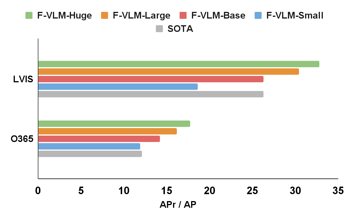 |
| F-VLM outperforms the state of the art (SOTA) on LVIS open-vocabulary detection benchmark and transfer object detection. On the x-axis, we show the LVIS metric mask AP on rare categories (APr), and the Objects365 (O365) metric box AP on all categories. The sizes of the detector backbones are as follows: Small(R50), Base (R50x4), Large(R50x16), Huge(R50x64). The naming follows CLIP convention. |
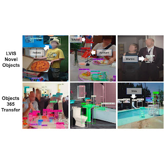
We visualize F-VLM on open-vocabulary detection and transfer detection tasks (shown below). On LVIS and Objects365, F-VLM correctly detects both novel and common objects. A key benefit of open-vocabulary detection is to test on out-of-distribution data with categories given by users on the fly. See the F-VLM paper for more visualization on LVIS, Objects365 and Ego4D datasets.
 |
| F-VLM open-vocabulary and transfer detections. Top: Open-vocabulary detection on LVIS. We only show the novel categories for clarity. Bottom: Transfer to Objects365 dataset shows accurate detection of many categories. Novel categories detected: fedora, martini, pennant, football helmet (LVIS); slide (Objects365). |
Training efficiency
We show that F-VLM can achieve top performance with much less computational resources in the table below. Compared to the state-of-the-art approach, F-VLM can achieve better performance with 226x fewer resources and 57x faster wall clock time. Apart from training resource savings, F-VLM has potential for substantial memory savings at training time by running the backbone in inference mode. The F-VLM system runs almost as fast as a standard detector at inference time, because the only addition is a single attention pooling layer on the detected region features.
| Method | APr | Training Epochs | Training Cost (per-core-hour) |
Training Cost Savings | ||||||||||
| SOTA | 26.3 | 460 | 8,000 | 1x | ||||||||||
| F-VLM | 32.8 | 118 | 565 | 14x | ||||||||||
| F-VLM | 31.0 | 14.7 | 71 | 113x | ||||||||||
| F-VLM | 27.7 | 7.4 | 35 | 226x |
We provide additional results using the shorter Detectron2 training recipes (12 and 36 epochs), and show similarly strong performance by using a frozen backbone. The default setting is marked in gray.
| Backbone | Large Scale Jitter | #Epochs | Batch Size | APr | ||||||||||
| R50 | 12 | 16 | 18.1 | |||||||||||
| R50 | 36 | 64 | 18.5 | |||||||||||
| R50 | ✓ | 100 | 256 | 18.6 | ||||||||||
| R50x64 | 12 | 16 | 31.9 | |||||||||||
| R50x64 | 36 | 64 | 32.6 | |||||||||||
| R50x64 | ✓ | 100 | 256 | 32.8 |
Conclusion
We present F-VLM – a simple open-vocabulary detection method which harnesses the power of frozen pre-trained large vision-language models to provide detection of novel objects. This is done without a need for knowledge distillation, detection-tailored pre-training, or weakly supervised learning. Our approach offers significant compute savings and obviates the need for image-level labels. F-VLM achieves the new state-of-the-art in open-vocabulary detection on the LVIS benchmark at system level, and shows very competitive transfer detection on other datasets. We hope this study can both facilitate further research in novel-object detection and help the community explore frozen VLMs for a wider range of vision tasks.
Acknowledgements
This work is conducted by Weicheng Kuo, Yin Cui, Xiuye Gu, AJ Piergiovanni, and Anelia Angelova. We would like to thank our colleagues at Google Research for their advice and helpful discussions.
AI-powered code suggestions and security scans in Amazon SageMaker notebooks using Amazon CodeWhisperer and Amazon CodeGuru
Amazon SageMaker comes with two options to spin up fully managed notebooks for exploring data and building machine learning (ML) models. The first option is fast start, collaborative notebooks accessible within Amazon SageMaker Studio—a fully integrated development environment (IDE) for machine learning. You can quickly launch notebooks in Studio, easily dial up or down the underlying compute resources without interrupting your work, and even share your notebook as a link in few clicks. In addition to creating notebooks, you can perform all the ML development steps to build, train, debug, track, deploy, and monitor your models in a single pane of glass in Studio. The second option is Amazon SageMaker notebook instances—a single, fully managed ML compute instance running notebooks in the cloud, offering you more control on your notebook configurations.
Today, we are excited to announce the availability of Amazon CodeWhisperer and Amazon CodeGuru Security extensions in SageMaker notebooks. These AI-powered extensions help accelerate ML development by offering code suggestions as you type, and ensure that your code is secure and follows AWS best practices.
In this post, we show how you can get started with Amazon CodeGuru Security and CodeWhisperer in Studio and SageMaker notebook instances.
Solution overview
The CodeWhisperer extension is an AI coding companion that provides developers with real-time code suggestions in notebooks. Individual developers can use CodeWhisperer for free in Studio and SageMaker notebook instances. The coding companion generates real-time single-line or full function code suggestions. It understands semantics and context in your code and can recommend suggestions built on AWS and development best practices, improving developer efficiency, quality, and speed.
The CodeGuru Security extension offers security and code quality scans for Studio and SageMaker notebook instances. This assists notebook users in detecting security vulnerabilities such as injection flaws, data leaks, weak cryptography, or missing encryption within the notebook cells. You can also detect many common issues that affect the readability, reproducibility, and correctness of computational notebooks, such as misuse of ML library APIs, invalid run order, and nondeterminism. When vulnerabilities or quality issues are identified in the notebook, CodeGuru generates recommendations that enable you to remediate those issues based on AWS security best practices.
In the following sections, we show how to install each of the extensions and discuss the capabilities of each, demonstrating how these tools can improve overall developer productivity.
Prerequisites
If this is your first time working with Studio, you first need to create a SageMaker domain. Additionally, make sure you have appropriate access to both CodeWhisperer and CodeGuru using AWS Identity and Access Management (IAM).
You can use these extensions in any AWS Region, but requests to CodeWhisperer will be served through the us-east-1 Region. Requests will be served to CodeGuru in the Region of the Studio domain and if CodeGuru is supported in the Region. For all non-supported Regions, the requests will be served through us-east-1.
Set up CodeWhisperer with SageMaker notebooks
In this section, we demonstrate how to set up CodeWhisperer with SageMaker Studio.
Update IAM permissions to use the extension
You can use the CodeWhisperer extension in any Region, but all requests to CodeWhisperer will be served through the us-east-1 Region.
To use the CodeWhisperer extension, ensure that you have the necessary permissions. On the IAM console, add the following policy to the SageMaker user execution role:
Install the CodeWhisperer extension
You can install the CodeWhisperer extension through the command line. In this section, we look at the steps involved. To get started, complete the following steps:
- On the File menu, choose New and Terminal.
- Run the following commands to install the extension:
Refresh your browser, and you will have successfully installed the CodeWhisperer extension.

Use CodeWhisperer in Studio
After we complete the installation steps, we can use CodeWhisperer by opening a new notebook or Python file. For our example we will open a sample Notebook.
You will see a toolbar at the bottom of your notebook called CodeWhisperer. This shows common shortcuts for CodeWhisperer along with the ability to pause code suggestions, open the code reference log, and get a link to the CodeWhisperer documentation.
The code reference log will flag or filter code suggestions that resemble open-source training data. Get the associated open-source project’s repository URL and license so that you can more easily review them and add attributions.

To get started, place your cursor in a code block in your notebook, and CodeWhisperer will begin to make suggestions .If you don’t see suggestions, press Alt+C in Windows or Option+C in Mac to manually invoke suggestions.

The following video shows how to use CodeWhisperer to read and perform descriptive statistics on a data file in Studio.
Use CodeWhisperer in SageMaker Notebook Instances
Complete the following steps to use CodeWhisperer in notebook instances:
- Navigate to your SageMaker notebook instance.
- Make sure you have attached the CodeWhisperer policy from earlier to the notebook instance IAM role.
- When the permissions are added, choose Open JupyterLab.

- Install the extension. by using a terminal, on the File menu, choose New and Terminal, and enter the following commands:
- Once the commands complete, on the File menu, choose Shut Down to restart our Jupyter Server.

- Refresh the browser window.
You will now see the CodeWhisperer extension installed and ready to use.

Let’s test it out in a Python file.
- On the File menu, choose New and Python File.
The following video shows how to create a function to convert a JSON file to a CSV.
Set up CodeGuru Security with SageMaker notebooks
In this section, we demonstrate how to set up CodeGuru Security with SageMaker Studio.
Update IAM permissions to use the extension
To use the CodeGuru Security extension, ensure that you have the necessary permissions. Complete the following steps to update permission policies with IAM:
- Preferred: On the IAM console, you can attach the
AmazonCodeGuruSecurityScanAccessmanaged policy to your IAM identities. This policy grants permissions that allow a user to work with scans, including creating scans, viewing scan information, and viewing scan findings. - For custom policies, enter the following permissions:
- Attach the policy to any user or role that will use the CodeGuru Security extension.
For more information, see Policies and permissions in IAM.
Install the CodeGuru Security extension
You can install the CodeGuru Security extension through the command line. To get started, complete the following steps:
- On the File menu, choose New and Terminal.
- Run the following commands to install the extension in the
condaenvironment:
Refresh your browser, and you will have successfully installed the CodeGuru extension.

Run a code scan
The following steps demonstrate running your first CodeGuru Security scan using an example file:
- Create a new notebook called
example.ipynbwith the following code for testing purposes:
The below code has intentionally incorporated common bad practices to showcase the capabilities of Amazon CodeGuru Security.
- Important: Please confirm that the CodeGuru-Security extension is installed and if the LSP server says
Fully initializedas shown below when you open your notebook.
If you don’t see the extension fully initialized, return to the previous section to install the extension and complete the installation steps.

- Initiate the scan. You can initiate a scan in one of the following ways:
- Choose any code cell in your file, then choose the lightbulb icon.

- Choose (right-click) any code cell in your file, then choose Run CodeGuru scan.

- Choose any code cell in your file, then choose the lightbulb icon.
When the scan is started, the scan status will show as CodeGuru: Scan in progress.

After a few seconds, when the scan is complete, the status will change to CodeGuru: Scan completed.

View and address findings
After the scan is finished, your code may have some underlined findings. Hover over the underlined code, and a pop-up window appears with a brief summary of the finding. To access additional details about the findings, right-click on any cell and choose Show diagnostics panel.
This will open a panel containing additional information and suggestions related to the findings, located at the bottom of the notebook file.

After making changes to your code based on the recommendations, you can rerun the scan to check if the issue has been resolved. It’s important to note that the scan findings will disappear after you modify your code, and you’ll need to rerun the scan to view them again.
Enable automatic code scans
Automatic scans are disabled by default. Optionally, you can enable automatic code scans and set the frequency and AWS Region for your scan runs. To enable automatic code scans, complete the following steps.
- In Studio, on the Settings menu, choose Advanced Settings Editor.

- For Auto scans, choose Enabled.
- Specify the scan frequency in seconds and the Region for your CodeGuru Security scan.
For our example, we configure CodeGuru to perform an automatic security scan every 240 seconds in the us-east-1 Region. You can modify this value for any region that CodeGuru Security is supported.

Conclusion
SageMaker Studio and SageMaker Notebook Instances now support AI-powered CodeWhisperer and CodeGuru extensions that help you write secure code faster. We encourage you to try out both extensions. To learn more about CodeGuru Security for SageMaker, refer to Get started with the Amazon CodeGuru Extension for JupyterLab and SageMaker Studio, and to learn more about CodeWhisperer for SageMaker, refer to Setting up CodeWhisperer with Amazon SageMaker Studio. Please share any feedback in the comments!
About the authors
 Raj Pathak is a Senior Solutions Architect and Technologist specializing in Financial Services (Insurance, Banking, Capital Markets) and Machine Learning. He specializes in Natural Language Processing (NLP), Large Language Models (LLM) and Machine Learning infrastructure and operations projects (MLOps).
 Gaurav Parekh is a Solutions Architect helping AWS customers build large scale modern architecture. His core area of expertise include Data Analytics, Networking and Technology strategy. Outside of work, Gaurav enjoys playing cricket, soccer and volleyball.
 Arkaprava De is a Senior Software Engineer at AWS. He has been at Amazon for over 7 years and is currently working on improving the Amazon SageMaker Studio IDE experience. You can find him on LinkedIn.
 Prashant Pawan Pisipati is a Principal Product Manager at Amazon Web Services (AWS). He has built various products across AWS and Alexa, and is currently focused on helping Machine Learning practitioners be more productive through AWS services.
On Privacy and Personalization in Federated Learning: A Retrospective on the US/UK PETs Challenge
TL;DR: We study the use of differential privacy in personalized, cross-silo federated learning (NeurIPS’22), explain how these insights led us to develop a 1st place solution in the US/UK Privacy-Enhancing Technologies (PETs) Prize Challenge, and share challenges and lessons learned along the way. If you are feeling adventurous, checkout the extended version of this post with more technical details!
How can we be better prepared for the next pandemic?
Patient data collected by groups such as hospitals and health agencies is a critical tool for monitoring and preventing the spread of disease. Unfortunately, while this data contains a wealth of useful information for disease forecasting, the data itself may be highly sensitive and stored in disparate locations (e.g., across multiple hospitals, health agencies, and districts).
In this post we discuss our research on federated learning, which aims to tackle this challenge by performing decentralized learning across private data silos. We then explore an application of our research to the problem of privacy-preserving pandemic forecasting—a scenario where we recently won a 1st place, $100k prize in a competition hosted by the US & UK governments—and end by discussing several directions of future work based on our experiences.
Part 1: Privacy, Personalization, and Cross-Silo Federated Learning
Federated learning (FL) is a technique to train models using decentralized data without directly communicating such data. Typically:
- a central server sends a model to participating clients;
- the clients train that model using their own local data and send back updated models; and
- the server aggregates the updates (e.g., via averaging, as in FedAvg)
and the cycle repeats. Companies like Apple and Google have deployed FL to train models for applications such as predictive keyboards, text selection, and speaker verification in networks of user devices.
However, while significant attention has been given to cross-device FL (e.g., learning across large networks of devices such as mobile phones), the area of cross-silo FL (e.g., learning across a handful of data silos such as hospitals or financial institutions) is relatively under-explored, and it presents interesting challenges in terms of how to best model federated data and mitigate privacy risks. In Part 1.1, we’ll examine a suitable privacy granularity for such settings, and in Part 1.2, we’ll see how this interfaces with model personalization, an important technique in handling data heterogeneity across clients.
1.1. How should we protect privacy in cross-silo federated learning?
Although the high-level federated learning workflow described above can help to mitigate systemic privacy risks, past work suggests that FL’s data minimization principle alone isn’t sufficient for data privacy, as the client models and updates can still reveal sensitive information.
This is where differential privacy (DP) can come in handy. DP provides both a formal guarantee and an effective empirical mitigation to attacks like membership inference and data poisoning. In a nutshell, DP is a statistical notion of privacy where we add randomness to a query on a “dataset” to create quantifiable uncertainty about whether any one “data point” has contributed to the query output. DP is typically measured by two scalars ((varepsilon, delta))—the smaller, the more private.
In the above, “dataset” and “data point” are in quotes because privacy granularity matters. In cross-device FL, it is common to apply “client-level DP” when training a model, where the federated clients (e.g., mobile phones) are thought of as “data points”. This effectively ensures that each participating client/mobile phone user remains private.
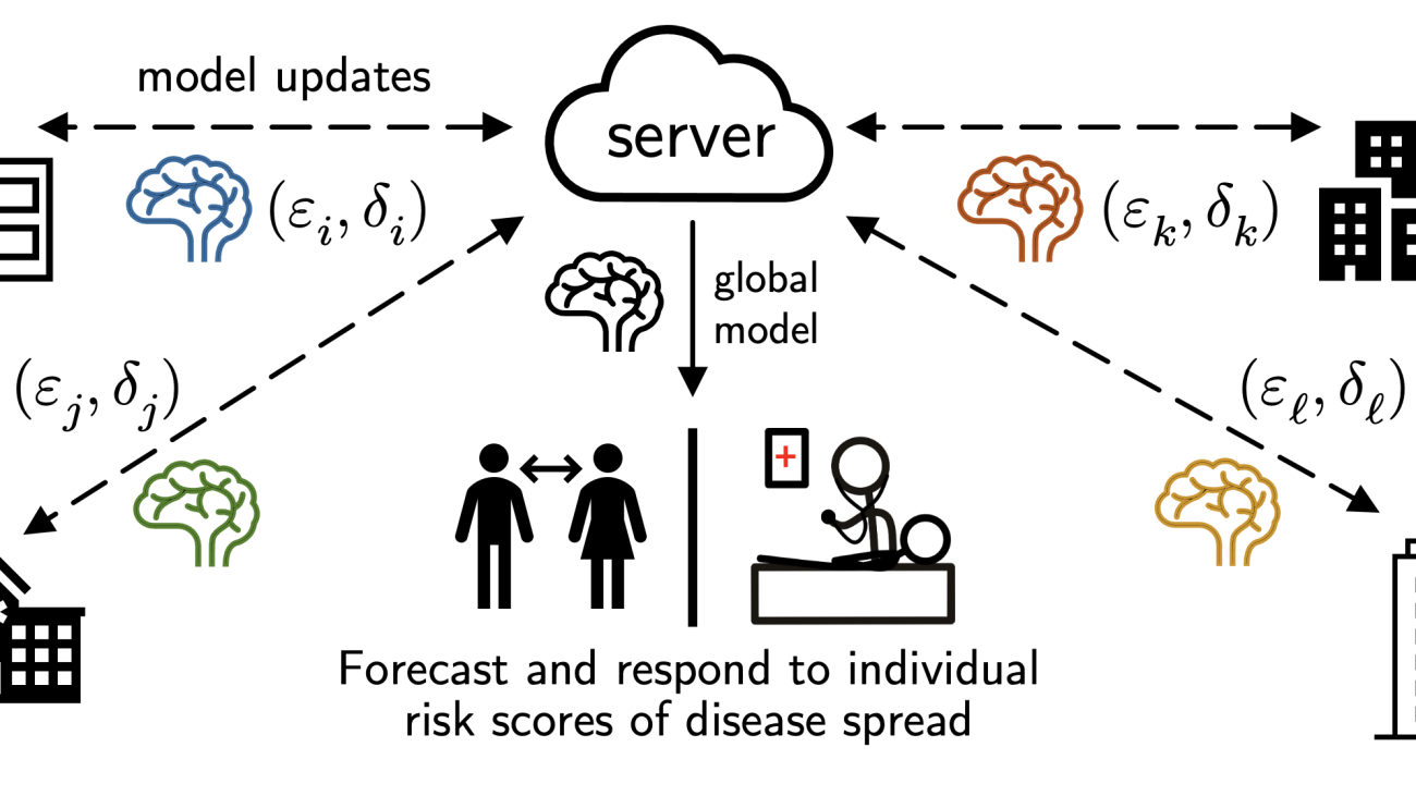
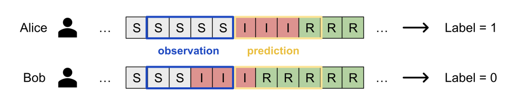
However, while client-level DP makes sense for cross-device FL as each client naturally corresponds to a person, this privacy granularity may not be suitable for cross-silo FL, where there are fewer (2-100) ‘clients’ but each holds many data subjects that require protection, e.g., each ‘client’ may be a hospital, bank, or school with many patient, customer, or student records.
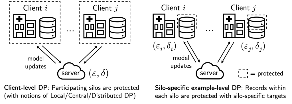
In our recent work (NeurIPS’22), we instead consider the notion of “silo-specific example-level DP” in cross-silo FL (see figure above). In short, this says that the (k)-th data silo may set its own ((varepsilon_k, delta_k)) example-level DP target for any learning algorithm with respect to its local dataset.
This notion is better aligned with real-world use cases of cross-silo FL, where each data subject contributes a single “example”, e.g., each patient in a hospital contributes their individual medical record. It is also very easy to implement: each silo can just run DP-SGD for local gradient steps with calibrated per-step noise. As we discuss below, this alternate privacy granularity affects how we consider modeling federated data to improve privacy/utility trade-offs.
1.2. The interplay of privacy, heterogeneity, and model personalization
Let’s now look at how this privacy granularity may interface with model personalization in federated learning.
Model personalization is a common technique used to improve model performance in FL when data heterogeneity (i.e. non-identically distributed data) exists between data silos.1 Indeed, existing benchmarks suggest that realistic federated datasets may be highly heterogeneous and that fitting separate local models on the federated data are already competitive baselines.
When considering model personalization techniques under silo-specific example-level privacy, we find that a unique trade-off may emerge between the utility costs from privacy and data heterogeneity (see figure below):
- As DP noises are added independently by each silo for its own privacy targets, these noises are reflected in the silos’ model updates and can thus be smoothed out when these updates are averaged (e.g. via FedAvg), leading to a smaller utility drop from DP for the federated model.
- On the other hand, federation also means that the shared, federated model may suffer from data heterogeneity (“one size does not fit all”).
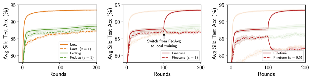
This “privacy-heterogeneity cost tradeoff” is interesting because it suggests that model personalization can play a key and distinct role in cross-silo FL. Intuitively, local training (no FL participation) and FedAvg (full FL participation) can be viewed as two ends of a personalization spectrum with identical privacy costs—silos’ participation in FL itself does not incur privacy costs due to DP’s robustness to post-processing—and various personalization algorithms (finetuning, clustering, …) are effectively navigating this spectrum in different ways.
If local training minimizes the effect of data heterogeneity but enjoys no DP noise reduction, and contrarily for FedAvg, it is natural to wonder whether there are personalization methods that lie in between and achieve better utility. If so, what methods would work best?
Our analysis points to mean-regularized multi-task learning (MR-MTL) as a simple yet particularly suitable form of personalization. MR-MTL simply asks each client (k) to train its own local model (w_k), regularize it towards the mean of others’ models (bar w) via a penalty (fraclambda 2 | w_k – bar w |_2^2 ), and keep (w_k) across rounds (i.e. client is stateful). The mean model (bar w) is maintained by the FL server (as in FedAvg) and may be updated in every round. More concretely, each local update step takes the following form:
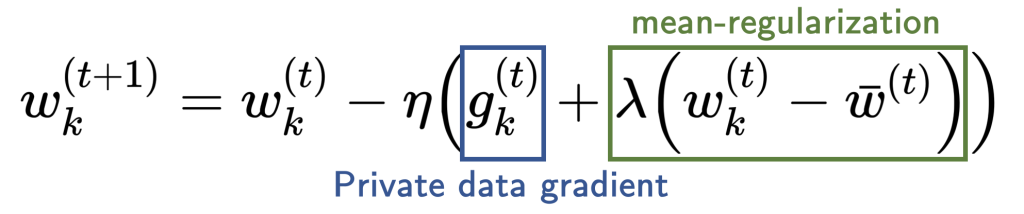
The hyperparameter (lambda) serves as a smooth knob between local training and FedAvg: (lambda = 0) recovers local training, and a larger (lambda) forces the personalized models to be closer to each other (intuitively, “federate more”).
MR-MTL has some nice properties in the context of private cross-silo FL:
- Noise reduction is attained throughout training via the soft proximity constraint towards an averaged model;
- The mean-regularization itself has no privacy overhead;2 and
- (lambda) provides a smooth interpolation along the personalization spectrum.
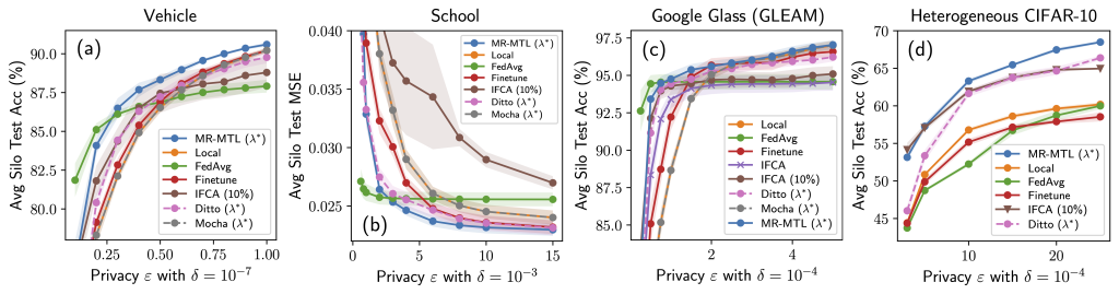
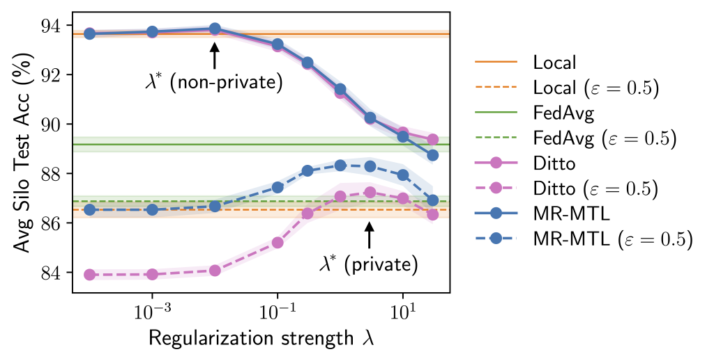
Why is the above interesting? Consider the following experiment where we try a range of (lambda) values roughly interpolating local training and FedAvg. Observe that we could find a “sweet spot” (lambda^ast) that outperforms both of the endpoints under the same privacy cost. Moreover, both the utility advantage of MR-MTL((lambda^ast)) over the endpoints, and (lambda^ast) itself, are larger under privacy; intuitively, this says that silos are encouraged to “federate more” for noise reduction.
The above provides rough intuition on why MR-MTL may be a strong baseline for private cross-silo FL and motivates this approach for a practical pandemic forecasting problem, which we discuss in Part 2. Our full paper delves deeper into the analyses and provides additional results and discussions!
Part 2: Federated Pandemic Forecasting at the US/UK PETs Challenge
Let’s now take a look at a federated pandemic forecasting problem at the US/UK Privacy-Enhancing Technologies (PETs) prize challenge, and how we may apply the ideas from Part 1.
2.1. Problem setup
The pandemic forecasting problem asks the following: Given a person’s demographic attributes (e.g. age, household size), locations, activities, infection history, and the contact network, what is the likelihood of infection in the next (t_text{pred}=7) days? Can we make predictions while protecting the privacy of individuals? Moreover, what if the data are siloed across administrative regions?
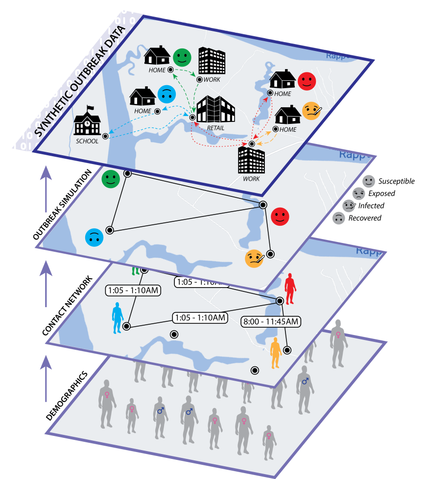
There’s a lot to unpack in the above. First, the pandemic outbreak problem follows a discrete-time SIR model (Susceptible → Infectious → Recovered) and we begin with a subset of the population infected. Subsequently,
- Each person goes about their usual daily activities and gets into contact with others (e.g. at a shopping mall)—this forms a contact graph where individuals are nodes and direct contacts are edges;
- Each person may get infected with different risk levels depending on a myriad of factors—their age, the nature and duration of their contact(s), their node centrality, etc.; and
- Such infection can also be asymptomatic—the individual can appear in the S state while being secretly infectious.
The challenge dataset models a pandemic outbreak in Virginia and contains roughly 7.7 million nodes (persons) and 186 million edges (contacts) with health states over 63 days; so the actual contact graph is fairly large but also quite sparse.
There are a few extra factors that make this problem challenging:
- Data imbalance: less than 5% of people are ever in the I or R state and roughly 0.3% of people became infected in the final week.
- Data silos: the true contact graph is cut along administrative boundaries, e.g., by grouped FIPS codes/counties. Each silo only sees a local subgraph, but people may still travel and make contacts across multiple regions! in In the official evaluation, the population sizes can also vary by more than 10(times) across silos.
- Temporal modeling: we are given the first (t_text{train} = 56) days of each person’s health states (S/I/R) and asked to predict individual infections any time in the subsequent ( t_text{pred} = 7 ) days. What is a training example in this case? How should we perform temporal partitioning? How does this relate to privacy accounting?
- Graphs generally complicate DP: we are often used to ML settings where we can clearly define the privacy granularity and how it relates to an actual individual (e.g. medical images of patients). This is tricky with graphs: people can make different numbers of contacts each of different natures, and their influence can propagate throughout the graph. At a high level (and as specified by the scope of sensitive data of the competition), what we care about is known as node-level DP—the model output is “roughly the same” if we add/remove/replace a node, along with its edges.
2.2. Applying MR-MTL with silo-specific example-level privacy
One clean approach to the pandemic forecasting problem is to just operate on the individual level and view it as (federated) binary classification: if we could build a feature vector to summarize an individual, then risk scores are simply the sigmoid probabilities of near-term infection.
Of course, the problem lies in what that feature vector (and the corresponding label) is—we’ll get to this in the following section. But already, we can see that MR-MTL with silo-specific example-level privacy (from Part 1) is a nice framework for a number of reasons:
- Model personalization is likely needed as the silos are large and heterogeneous by construction (geographic regions are unlike to all be similar).
- Privacy definition: There are a small number of clients, but each holds many data subjects, and client-level DP isn’t suitable.
- Usability, efficiency, and scalability: MR-MTL is remarkably easy to implement with minimal resource overhead (over FedAvg and local training). This is crucial for real-world applications.
- Adaptability and explainability: The framework is highly adaptable to any learning algorithm that can take DP-SGD-style updates. It also preserves the explainability of the underlying ML algorithm as we don’t obfuscate the model weights, updates, or predictions.
It is also helpful to look at the threat model we might be dealing with and how our framework behaves under it; the interested reader may find more details in the extended post!
2.3. Building training examples
We now describe how to convert individual information and the contact network into a tabular dataset for every silo ( k ) with ( n_k ) nodes.
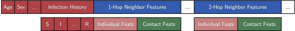
Recall that our task is to predict the risk of infection of a person within ( t_text{pred} = 7) days, and that each silo only sees its local subgraph. We formulate this via a silo-specific set of examples ( ( X_k in mathbb R^{n_k times d}, Y_k in mathbb {0, 1}^{n_k} ) ), where the features ( {X_k^{(i)} in mathbb R^d} ) describe the neighborhood around a person ( i ) (see figure) and binary label ( {Y_k^{(i)}} ) denotes if the person become infected in the next ( t_text{pred} ) days.
Each example’s features ( X_k^{(i)} ) consist of the following:
(1) Individual features: Basic (normalized) demographic features like age, gender, and household size; activity features like working, school, going to church, or shopping; and the individual’s infection history as concatenated one-hot vectors (which depends on how we create labels; see below).
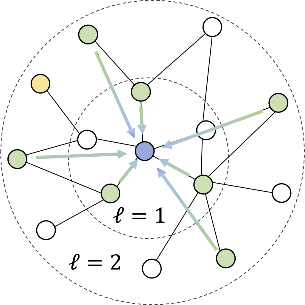
(2) Contact features: One of our key simplifying heuristics is that each node’s (ell)-hop neighborhood should contain most of the information we need to predict infection. We build the contact features as follows:
- Every sampled neighbor (v) of a node (u) is encoded using its individual features (as above) along with the edge features describing the contact—e.g. the location, the duration, and the activity type.
- We use iterative neighborhood sampling (figure above), meaning that we first select a set of ( S_1 ) 1-hop neighbors, and then sample (S_2) 2-hop neighbors adjacent to those 1-hop neighbors, and so on. This allows reusing 1-hop edge features and keeps the feature dimension (d) low.
- We also used deterministic neighborhood sampling—the same person always takes the same subset of neighbors. This drastically reduces computation as the graph/neighborhoods can now be cached. For the interested reader, this also has implications on privacy accounting.
The figure above illustrates the neighborhood feature vector that describes a person and their contacts for the binary classifier! Intriguingly, this makes the per-silo models a simplified variant of a graph neural network (GNN) with a single-step, non-parameterized neighborhood aggregation and prediction (cf. SGC models).
For the labels ( Y_k^{(i)} ), we deployed a random infection window strategy:
- Pick a window size ( t_text{window} ) (say 21 days);
- Select a random day (t’) within the valid range ((t_text{window} le t’ le t_text{train} – t_text{pred}));
- Encode the S/I/R states in the past window from (t’) for every node in the neighborhood as individual features;
- The label is then whether person (i) is infected in any of the next (t_text{pred}) days from (t’).
Our strategy implicitly assumes that a person’s infection risk is individual: whether Bob gets infected depends only on his own activities and contacts in the past window. This is certainly not perfect as it ignores population-level modeling (e.g. denser areas have higher risks of infection), but it makes the ML problem very simple: just plug-in existing tabular data modeling approaches!
2.4. Putting it all together
We can now see our solution coming together: each silo builds a tabular dataset using neighborhood vectors for features and infection windows for labels, and each silo trains a personalized binary classifier under MR-MTL with silo-specific example-level privacy. We complete our method with a few additional ingredients:
- Privacy accounting. We’ve so far glossed over what silo-specific “example-level” DP actually means for an individual. We’ve put more details in the extended blog post, and the main idea is that local DP-SGD can give “neighborhood-level” DP since each node’s enclosing neighborhood is fixed and unique, and we can then convert it to node-level DP (our privacy goal from Part 2.1) by carefully accounting for how a certain node may appear in other nodes’ neighborhoods.
- Noisy SGD as an empirical defense. While we have a complete framework for providing silo-specific node-level DP guarantees, for the PETs challenge specifically we decided to opt for weak DP ((varepsilon > 500)) as an empirical protection, rather than a rigorous theoretical guarantee. While some readers may find this mildly disturbing at first glance, we note that the strength of protection depends on the data, the models, the actual threats, the desired privacy-utility trade-off, and several crucial factors linking theory and practice which we outline in the extended blog. Our solution was in turn attacked by several red teams to test for vulnerabilities.
- Model architecture: simple is good. While the model design space is large, we are interested in methods amenable to gradient-based private optimization (e.g. DP-SGD) and weight-space averaging for federated learning. We compared simple logistic regression and a 3-layer MLP and found that the variance in data strongly favors linear models, which also have benefits in privacy (in terms of limited capacity for memorization) as well as explainability, efficiency, and robustness.
- Computation-utility tradeoff for neighborhood sampling. While larger neighborhood sizes (S) and more hops (ell) better capture the original contact graph, they also blow up the computation and our experiments found that larger (S) and (ell) tend to have diminishing returns.
- Data imbalance and weighted loss. Because the data are highly imbalanced, training naively will suffer from low recall and AUPRC. While there are established over-/under-sampling methods to deal with such imbalance, they, unfortunately, make privacy accounting a lot trickier in terms of the subsampling assumption or the increased data queries. We leveraged the focal loss from the computer vision literature designed to emphasize hard examples (infected cases) and found that it did improve both the AUPRC and the recall considerably.
The above captures the essence of our entry to the challenge. Despite the many subtleties in fully building out a working system, the main ideas were quite simple: train personalized models with DP and add some proximity constraints!
Takeaways and Open Challenges
In Part 1, we reviewed our NeurIPS’22 paper that studied the application of differential privacy in cross-silo federated learning scenarios, and in Part 2, we saw how the core ideas and methods from the paper helped us develop our submission to the PETs prize challenge and win a 1st place in the pandemic forecasting track. For readers interested in more details—such as theoretical analyses, hyperparameter tuning, further experiments, and failure modes—please check out our full paper. Our work also identified several important future directions in this context:
DP under data imbalance. DP is inherently a uniform guarantee, but data imbalance implies that examples are not created equal—minority examples (e.g., disease infection, credit card fraud) are more informative, and they tend to give off (much) larger gradients during model training. Should we instead do class-specific (group-wise) DP or refine “heterogeneous DP” or “outlier DP” notions to better cater to the discrepancy between data points?
Graphs and privacy. Another fundamental basis of DP is that we could delineate what is and isn’t an individual. But as we’ve seen, the information boundaries are often nebulous when an individual is a node in a graph (think social networks and gossip propagation), particularly when the node is arbitrarily well connected. Instead of having rigid constraints (e.g., imposing a max node degree and accounting for it), are there alternative privacy definitions that offer varying degrees of protection for varying node connectedness?
Scalable, private, and federated trees for tabular data. Decision trees/forests tend to work extremely well for tabular data such as ours, even with data imbalance, but despite recent progress, we argue that they are not yet mature under private and federated settings due to some underlying assumptions.
Novel training frameworks. While MR-MTL is a simple and strong baseline under our privacy granularity, it has clear limitations in terms of modeling capacity. Are there other methods that can also provide similar properties to balance the emerging privacy-heterogeneity cost tradeoff?
Honest privacy cost of hyperparameter search. When searching for better frameworks, the dependence on hyperparameters is particularly interesting: our full paper (section 7) made a surprising but somewhat depressing observation that the honest privacy cost of just tuning (on average) 10 configurations (values of (lambda) in this case) may already outweigh the utility advantage of the best tune MR-MTL((lambda^ast)). What does this mean if MR-MTL is already a strong baseline with just a single hyperparameter?
Check out the following related links:
- Extended version of this blog with more technical details
- Part 1: Our NeurIPS’22 paper and poster
- Part 2: The US/UK Privacy-Enhancing Technologies (PETs) Prize Challenge
- Team profile
- Open-source release
- Description: challenge main page, technical brief of the federated pandemic forecasting problem
- News coverage: DrivenData, CMU, White House, NSF, UK Gov
DISCLAIMER: All opinions expressed in this post are those of the authors and do not represent the views of CMU.
Footnotes
1 Note that “personalization” refers to customizing models for each client (data silo) in federated learning rather than for a specific person.
2 As compared to local training or FedAvg for a fixed (lambda). However, tuning (lambda) as a hyperparameter can incur privacy cost.

Enabling conversational interaction on mobile with LLMs
Intelligent assistants on mobile devices have significantly advanced language-based interactions for performing simple daily tasks, such as setting a timer or turning on a flashlight. Despite the progress, these assistants still face limitations in supporting conversational interactions in mobile user interfaces (UIs), where many user tasks are performed. For example, they cannot answer a user’s question about specific information displayed on a screen. An agent would need to have a computational understanding of graphical user interfaces (GUIs) to achieve such capabilities.
Prior research has investigated several important technical building blocks to enable conversational interaction with mobile UIs, including summarizing a mobile screen for users to quickly understand its purpose, mapping language instructions to UI actions and modeling GUIs so that they are more amenable for language-based interaction. However, each of these only addresses a limited aspect of conversational interaction and requires considerable effort in curating large-scale datasets and training dedicated models. Furthermore, there is a broad spectrum of conversational interactions that can occur on mobile UIs. Therefore, it is imperative to develop a lightweight and generalizable approach to realize conversational interaction.
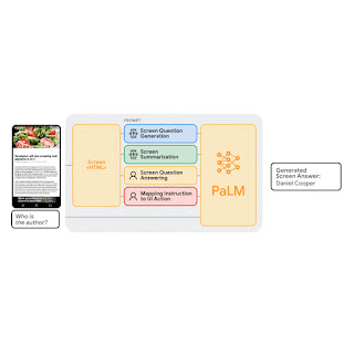
In “Enabling Conversational Interaction with Mobile UI using Large Language Models”, presented at CHI 2023, we investigate the viability of utilizing large language models (LLMs) to enable diverse language-based interactions with mobile UIs. Recent pre-trained LLMs, such as PaLM, have demonstrated abilities to adapt themselves to various downstream language tasks when being prompted with a handful of examples of the target task. We present a set of prompting techniques that enable interaction designers and developers to quickly prototype and test novel language interactions with users, which saves time and resources before investing in dedicated datasets and models. Since LLMs only take text tokens as input, we contribute a novel algorithm that generates the text representation of mobile UIs. Our results show that this approach achieves competitive performance using only two data examples per task. More broadly, we demonstrate LLMs’ potential to fundamentally transform the future workflow of conversational interaction design.
 |
| Animation showing our work on enabling various conversational interactions with mobile UI using LLMs. |
Prompting LLMs with UIs
LLMs support in-context few-shot learning via prompting — instead of fine-tuning or re-training models for each new task, one can prompt an LLM with a few input and output data exemplars from the target task. For many natural language processing tasks, such as question-answering or translation, few-shot prompting performs competitively with benchmark approaches that train a model specific to each task. However, language models can only take text input, while mobile UIs are multimodal, containing text, image, and structural information in their view hierarchy data (i.e., the structural data containing detailed properties of UI elements) and screenshots. Moreover, directly inputting the view hierarchy data of a mobile screen into LLMs is not feasible as it contains excessive information, such as detailed properties of each UI element, which can exceed the input length limits of LLMs.
To address these challenges, we developed a set of techniques to prompt LLMs with mobile UIs. We contribute an algorithm that generates the text representation of mobile UIs using depth-first search traversal to convert the Android UI’s view hierarchy into HTML syntax. We also utilize chain of thought prompting, which involves generating intermediate results and chaining them together to arrive at the final output, to elicit the reasoning ability of the LLM.
 |
| Animation showing the process of few-shot prompting LLMs with mobile UIs. |
Our prompt design starts with a preamble that explains the prompt’s purpose. The preamble is followed by multiple exemplars consisting of the input, a chain of thought (if applicable), and the output for each task. Each exemplar’s input is a mobile screen in the HTML syntax. Following the input, chains of thought can be provided to elicit logical reasoning from LLMs. This step is not shown in the animation above as it is optional. The task output is the desired outcome for the target tasks, e.g., a screen summary or an answer to a user question. Few-shot prompting can be achieved with more than one exemplar included in the prompt. During prediction, we feed the model the prompt with a new input screen appended at the end.
Experiments
We conducted comprehensive experiments with four pivotal modeling tasks: (1) screen question-generation, (2) screen summarization, (3) screen question-answering, and (4) mapping instruction to UI action. Experimental results show that our approach achieves competitive performance using only two data examples per task.
 |
Task 1: Screen question generation
Given a mobile UI screen, the goal of screen question-generation is to synthesize coherent, grammatically correct natural language questions relevant to the UI elements requiring user input.
We found that LLMs can leverage the UI context to generate questions for relevant information. LLMs significantly outperformed the heuristic approach (template-based generation) regarding question quality.
 |
| Example screen questions generated by the LLM. The LLM can utilize screen contexts to generate grammatically correct questions relevant to each input field on the mobile UI, while the template approach falls short. |
We also revealed LLMs’ ability to combine relevant input fields into a single question for efficient communication. For example, the filters asking for the minimum and maximum price were combined into a single question: “What’s the price range?
 |
| We observed that the LLM could use its prior knowledge to combine multiple related input fields to ask a single question. |
In an evaluation, we solicited human ratings on whether the questions were grammatically correct (Grammar) and relevant to the input fields for which they were generated (Relevance). In addition to the human-labeled language quality, we automatically examined how well LLMs can cover all the elements that need to generate questions (Coverage F1). We found that the questions generated by LLM had almost perfect grammar (4.98/5) and were highly relevant to the input fields displayed on the screen (92.8%). Additionally, LLM performed well in terms of covering the input fields comprehensively (95.8%).
| Template | 2-shot LLM | |||||||
| Grammar | 3.6 (out of 5) | 4.98 (out of 5) | ||||||
| Relevance | 84.1% | 92.8% | ||||||
| Coverage F1 | 100% | 95.8% |
Task 2: Screen summarization
Screen summarization is the automatic generation of descriptive language overviews that cover essential functionalities of mobile screens. The task helps users quickly understand the purpose of a mobile UI, which is particularly useful when the UI is not visually accessible.
Our results showed that LLMs can effectively summarize the essential functionalities of a mobile UI. They can generate more accurate summaries than the Screen2Words benchmark model that we previously introduced using UI-specific text, as highlighted in the colored text and boxes below.
 |
| Example summary generated by 2-shot LLM. We found the LLM is able to use specific text on the screen to compose more accurate summaries. |
Interestingly, we observed LLMs using their prior knowledge to deduce information not presented in the UI when creating summaries. In the example below, the LLM inferred the subway stations belong to the London Tube system, while the input UI does not contain this information.
 |
| LLM uses its prior knowledge to help summarize the screens. |
Human evaluation rated LLM summaries as more accurate than the benchmark, yet they scored lower on metrics like BLEU. The mismatch between perceived quality and metric scores echoes recent work showing LLMs write better summaries despite automatic metrics not reflecting it.
 |
 |
| Left: Screen summarization performance on automatic metrics. Right: Screen summarization accuracy voted by human evaluators. |
Task 3: Screen question-answering
Given a mobile UI and an open-ended question asking for information regarding the UI, the model should provide the correct answer. We focus on factual questions, which require answers based on information presented on the screen.
 |
| Example results from the screen QA experiment. The LLM significantly outperforms the off-the-shelf QA baseline model. |
We report performance using four metrics: Exact Matches (identical predicted answer to ground truth), Contains GT (answer fully containing ground truth), Sub-String of GT (answer is a sub-string of ground truth), and the Micro-F1 score based on shared words between the predicted answer and ground truth across the entire dataset.
Our results showed that LLMs can correctly answer UI-related questions, such as “what’s the headline?”. The LLM performed significantly better than baseline QA model DistillBERT, achieving a 66.7% fully correct answer rate. Notably, the 0-shot LLM achieved an exact match score of 30.7%, indicating the model’s intrinsic question answering capability.
| Models | Exact Matches | Contains GT | Sub-String of GT | Micro-F1 | ||||||||||
| 0-shot LLM | 30.7% | 6.5% | 5.6% | 31.2% | ||||||||||
| 1-shot LLM | 65.8% | 10.0% | 7.8% | 62.9% | ||||||||||
| 2-shot LLM | 66.7% | 12.6% | 5.2% | 64.8% | ||||||||||
| DistillBERT | 36.0% | 8.5% | 9.9% | 37.2% |
Task 4: Mapping instruction to UI action
Given a mobile UI screen and natural language instruction to control the UI, the model needs to predict the ID of the object to perform the instructed action. For example, when instructed with “Open Gmail,” the model should correctly identify the Gmail icon on the home screen. This task is useful for controlling mobile apps using language input such as voice access. We introduced this benchmark task previously.
 |
| Example using data from the PixelHelp dataset. The dataset contains interaction traces for common UI tasks such as turning on wifi. Each trace contains multiple steps and corresponding instructions. |
We assessed the performance of our approach using the Partial and Complete metrics from the Seq2Act paper. Partial refers to the percentage of correctly predicted individual steps, while Complete measures the portion of accurately predicted entire interaction traces. Although our LLM-based method did not surpass the benchmark trained on massive datasets, it still achieved remarkable performance with just two prompted data examples.
| Models | Partial | Complete | ||||||
| 0-shot LLM | 1.29 | 0.00 | ||||||
| 1-shot LLM (cross-app) | 74.69 | 31.67 | ||||||
| 2-shot LLM (cross-app) | 75.28 | 34.44 | ||||||
| 1-shot LLM (in-app) | 78.35 | 40.00 | ||||||
| 2-shot LLM (in-app) | 80.36 | 45.00 | ||||||
| Seq2Act | 89.21 | 70.59 |
Takeaways and conclusion
Our study shows that prototyping novel language interactions on mobile UIs can be as easy as designing a data exemplar. As a result, an interaction designer can rapidly create functioning mock-ups to test new ideas with end users. Moreover, developers and researchers can explore different possibilities of a target task before investing significant efforts into developing new datasets and models.
We investigated the feasibility of prompting LLMs to enable various conversational interactions on mobile UIs. We proposed a suite of prompting techniques for adapting LLMs to mobile UIs. We conducted extensive experiments with the four important modeling tasks to evaluate the effectiveness of our approach. The results showed that compared to traditional machine learning pipelines that consist of expensive data collection and model training, one could rapidly realize novel language-based interactions using LLMs while achieving competitive performance.
Acknowledgements
We thank our paper co-author Gang Li, and appreciate the discussions and feedback from our colleagues Chin-Yi Cheng, Tao Li, Yu Hsiao, Michael Terry and Minsuk Chang. Special thanks to Muqthar Mohammad and Ashwin Kakarla for their invaluable assistance in coordinating data collection. We thank John Guilyard for helping create animations and graphics in the blog.
NerfDiff: Single-image View Synthesis with NeRF-guided Distillation from 3D-aware Diffusion
Novel view synthesis from a single image requires inferring occluded regions of objects and scenes while simultaneously maintaining semantic and physical consistency with the input. Existing approaches condition neural radiance fields (NeRF) on local image features, projecting points to the input image plane, and aggregating 2D features to perform volume rendering. However, under severe occlusion, this projection fails to resolve uncertainty, resulting in blurry renderings that lack details. In this work, we propose NerfDiff, which addresses this issue by distilling the knowledge of a 3D-aware…Apple Machine Learning Research
Unlock Insights from your Amazon S3 data with intelligent search
Amazon Kendra is an intelligent search service powered by machine learning (ML). Amazon Kendra reimagines enterprise search for your websites and applications so your employees and customers can easily find the content they’re looking for, even when it’s scattered across multiple locations and content repositories within your organization. Keywords or natural language questions can be used to search most relevant documents powered by ML to deliver answers and rank documents. Amazon Kendra can index data from Amazon Simple Storage Service (Amazon S3) or from a third-party document repository. Amazon S3 is an object storage service that offers scalability and availability where you can store large amounts of data, including product manuals, project and research documents, and more.
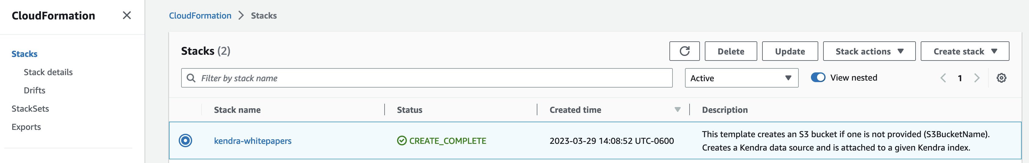
In this post, you can learn how to deploy a provided AWS CloudFormation template to index your documents in an Amazon S3 bucket. The template creates an Amazon Kendra data source for an index and synchronizes your data source according to your needs: on-demand, hourly, daily, weekly or monthly. AWS CloudFormation allows us to provision infrastructure as code (IaC) so you can spend less time managing resources, replicate your infrastructure quickly, and control and track changes in the infrastructure.
Overview of the solution
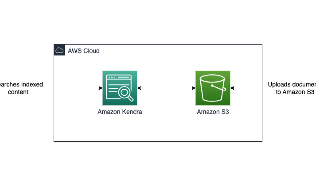
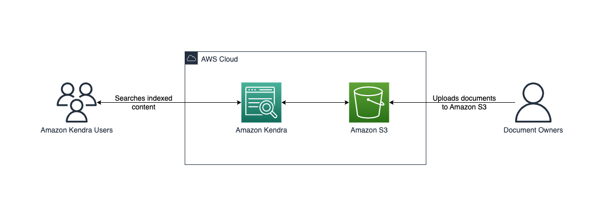
The CloudFormation template sets up an Amazon Kendra data source with a connection to Amazon S3. The template also creates one role for the Amazon Kendra data source service. You can specify an S3 bucket, synchronization schedule, and inclusion/exclusion patterns. When the synchronization job has finished, you can search the indexed content through the Search console. The following diagram illustrates this workflow.
This post guides you to the following steps:
- Deploy the provided template.
- Upload the documents to the S3 bucket that you create. If you provide a bucket with documents, you can omit this step.
- Wait until the index finishes crawling the data source.
Prerequisites
For this walkthrough, you should have the following prerequisites:
- An AWS account where the proposed solution can be deployed.
- An Amazon Kendra index for attaching a data source to the stack.
- The set of documents that are used to create the Amazon Kendra index. In this solution, you are using a compressed file of AWS whitepapers.
Deploy the solution with AWS CloudFormation
To deploy the CloudFormation template, complete the following steps:
- Choose

You’re redirected to the AWS CloudFormation console.
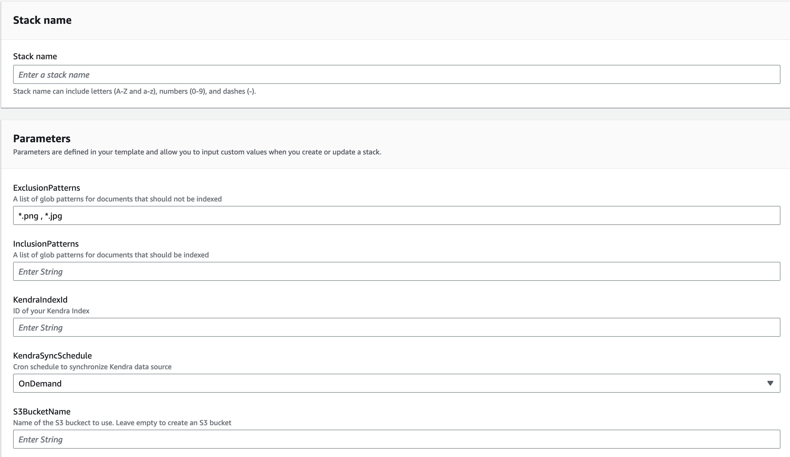
- You can modify the parameters or use the default values:
- The Amazon Kendra data source name is automatically set using the stack name and associated bucket name.
- For KendraIndexId, enter the Amazon Kendra index ID where you will attach the data source.
- You can also choose when you want to run the data source synchronization using KendraSyncSchedule. By default, it’s set to OnDemand.
- For S3BucketName, you can either enter a bucket you have already created or leave it empty. If you leave it empty, a bucket will be created for you. Either way, the bucket is used as the Amazon Kendra data source. For this post, we leave it empty.
It takes around 5 minutes for the stack to deploy the Amazon Kendra data source attached to the Amazon Kendra index.
- On the Outputs tab of the CloudFormation stack, copy the name of the created bucket, data source name, and ID.
The created stack deploys one role: <stack-name>-KendraDataSourceRole. It’s a best practice to deploy a role for each data source you create. This role gives Amazon Kendra data source to add or remove files from Amazon Kendra index, to get objects from Amazon S3 bucket.
Upload files to the S3 bucket
Amazon Kendra can handle multiple document types, such as .html, .pdf, .csv, .json, .docx, and .ppt. You can also have a combination of documents on a single index. The text contained in those documents is indexed to the provided Amazon Kendra index. You can search for keywords on AWS topics on best practices, databases, machine learning, security, and more using over 60 pdf files that you can download. For example, if you want to know where you can find more information about caching in the AWS whitepapers, Amazon Kendra can help you find documents related to databases and best practices.
When you download the AWS Whitepapers.zip file and uncompress the file, you see these six folders: Best_Practices, Databases, General, Machine_Learning, Security, Well_Architected. Upload these folders to your S3 bucket.

Synchronize the Amazon Kendra data source
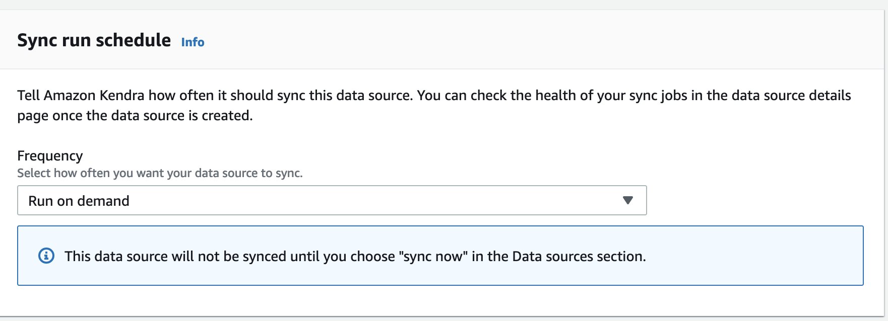
Amazon Kendra data source data can synchronize your data based on preconfigured schedule or can be be manually triggered on-demand. By default, CloudFormation template configures the data source to on-demand synchronization schedule to be triggered manually as required.
To manually trigger the synchronization job from the AWS Amazon Kendra console, navigate to the Amazon Kendra index used as part of CloudFormation stack deployment, under Data Management in the navigation pane, choose Data Sources and then choose Sync now. This makes the S3 bucket synchronize with the data source.
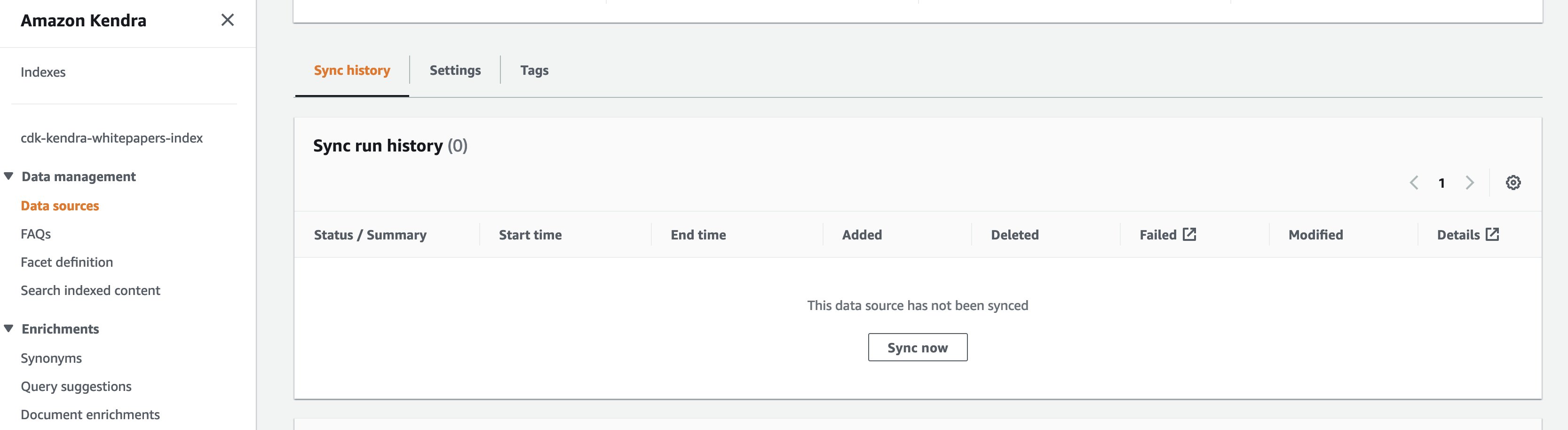
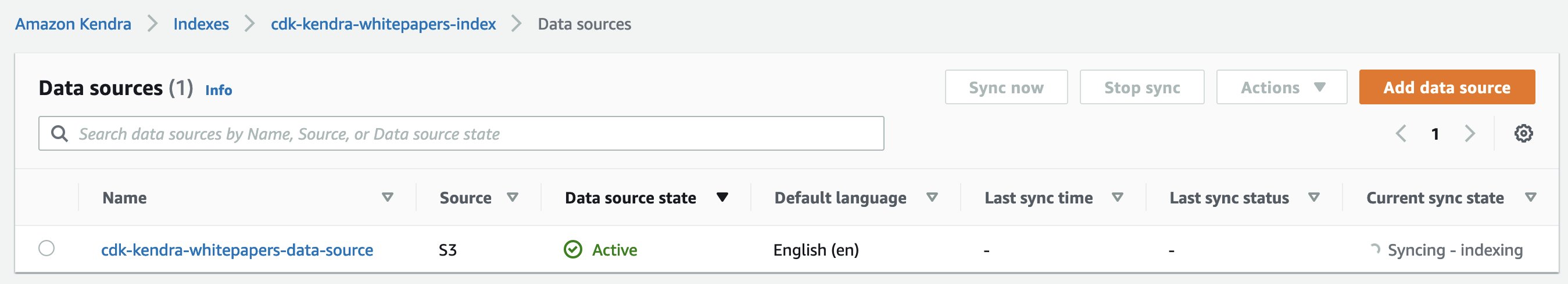
When the Amazon Kendra data source starts syncing, you should see the Current sync state as Syncing.
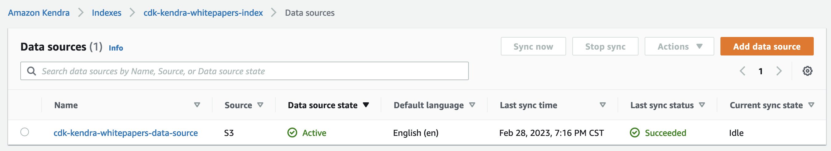
When the data source has finished, the Last sync status appears as Succeeded and Current sync state as Idle. You can now search the indexed content.
Configure synchronization schedule
The template allows you to run the schedule every hour at minute 0, for example, 13:00, 14:00, or 15:00. You also have the option to run it daily at 00:00 UTC. The Weekly setting runs Mondays at 00:00 UTC, and the Monthly setting runs every first day of the month at 00:00 UTC.
To change the schedule after the Amazon Kendra data source has been created, on the Actions menu, choose Edit. Under Configure sync settings, you find the Sync rule schedule section.
Under Frequency, you can select hourly, daily, weekly, monthly, or custom, all of which allow you to schedule your sync down to the minute.
Add exclusion patterns
The provided CloudFormation template allows you to add exclusion patterns. By default, .png and .jpg files will be added to the ExclusionPatterns parameter. Additional file formats can be added as a comma separated list to the exclusion pattern. Similarly, InclusionPatterns parameter may be used add comma list file formats to set up an inclusion pattern. If you don’t provide an inclusion pattern, all files are indexed except for the ones included in the exclusion parameter.
Clean up
To avoid costs, you can delete the stack from the AWS CloudFormation console. On the Stacks page, select the stack you created, choose Delete, and confirm the deletion of the stack.
If you haven’t provided a S3 bucket, the stack creates a bucket. If the bucket is empty, it’s automatically deleted. Otherwise, you need to empty the folder and manually delete it. If you provided a bucket, even if it’s empty, it won’t be deleted. Amazon Kendra index won’t be deleted. Only the Amazon Kendra data source created by the stack will be deleted.
Conclusion
In this post, we provided an CloudFormation template to easily synchronize your text documents on an S3 bucket to your Amazon Kendra index. This solution is helpful if you have multiple S3 buckets you want to index because you can create all the necessary components to query the documents with a few clicks in a consistent and repeatable manner. You can also see how image-based text documents can be handled in Amazon Kendra. To learn more about specific schedule patterns, refer to Schedule Expressions for Rules.
Leave a comment and learn more about Amazon Kendra index creation in the following Amazon Kendra Essentials+ workshop.
Special thanks to Jose Mauricio Mani Yanez for his help creating the example code and compiling the content for this post.
About the author
 Rajesh Kumar Ravi is an AI/ML Specialist Solutions Architect at Amazon Web Services specializing in intelligent document search with Amazon Kendra and generative AI. He is a builder and problem solver, and contributes to development of new ideas. He enjoys walking and loves to go on short hiking trips outside of work.
Language Identification: Building an End-to-End AI Solution using PyTorch
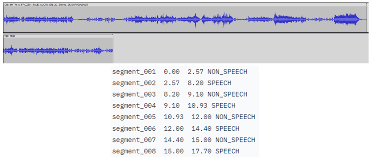
Language Identification is the process of identifying the primary language from multiple audio input samples. In natural language processing (NLP), language identification is an important problem and a challenging issue. There are many language-related tasks such as entering text on your phone, finding news articles you enjoy, or discovering answers to questions that you may have. All these tasks are powered by NLP models. To decide which model to invoke at a particular point in time, we must perform language identification.
This article presents an in-depth solution and code sample for language identification using Intel® Extension for PyTorch, which is a version of the popular PyTorch AI framework optimized for use on Intel® processors, and Intel® Neural Compressor, which is a tool to accelerate AI inference without sacrificing accuracy.
The code sample demonstrates how to train a model to perform language identification using the Hugging Face SpeechBrain* toolkit and optimize it using the Intel® AI Analytics Toolkit (AI Kit). The user can modify the code sample and identify up to 93 languages using the Common Voice dataset.
Proposed Methodology for Language Identification
In the proposed solution, the user will use an Intel AI Analytics Toolkit container environment to train a model and perform inference leveraging Intel-optimized libraries for PyTorch. There is also an option to quantize the trained model with Intel Neural Compressor to speed up inference.
Dataset
The Common Voice dataset is used and for this code sample, specifically, Common Voice Corpus 11.0 for Japanese and Swedish. This dataset is used to train an Emphasized Channel Attention, Propagation and Aggregation Time Delay Neural Network (ECAPA-TDNN), which is implemented using the Hugging Face SpeechBrain library. Time Delay Neural Networks (TDNNs), aka one-dimensional Convolutional Neural Networks (1D CNNs), are multilayer artificial neural network architectures to classify patterns with shift-invariance and model context at each layer of the network. ECAPA-TDNN is a new TDNN-based speaker-embedding extractor for speaker verification; it is built upon the original x-vector architecture and puts more emphasis on channel attention, propagation, and aggregation.
Implementation
After downloading the Common Voice dataset, the data is preprocessed by converting the MP3 files into WAV format to avoid information loss and separated into training, validation, and testing sets.
A pretrained VoxLingua107 model is retrained with the Common Voice dataset using the Hugging Face SpeechBrain library to focus on the languages of interest. VoxLingua107 is a speech dataset used for training spoken language recognition models that work well with real-world and varying speech data. This dataset contains data for 107 languages. By default, Japanese and Swedish are used, and more languages can be included. This model is then used for inference on the testing dataset or a user-specified dataset. Also, there is an option to utilize SpeechBrain’s Voice Activity Detection (VAD) where only the speech segments from the audio files are extracted and combined before samples are randomly selected as input into the model. This link provides all the necessary tools to perform VAD. To improve performance, the user may quantize the trained model to integer-8 (INT8) using Intel Neural Compressor to decrease latency.
Training
The copies of training scripts are added to the current working directory, including create_wds_shards.py – for creating the WebDataset shards, train.py – to perform the actual training procedure, and train_ecapa.yaml – to configure the training options. The script to create WebDataset shards and YAML file are patched to work with the two languages chosen for this code sample.
In the data preprocessing phase, prepareAllCommonVoice.py script is executed to randomly select a specified number of samples to convert the input from MP3 to WAV format. Here, 80% of these samples will be used for training, 10% for validation, and 10% for testing. At least 2000 samples are recommended as the number of input samples and is the default value.
In the next step, WebDataset shards are created from the training and validation datasets. This stores the audio files as tar files which allows writing purely sequential I/O pipelines for large-scale deep learning in order to achieve high I/O rates from local storage—about 3x-10x faster compared to random access.
The YAML file will be modified by the user. This includes setting the value for the largest number for the WebDataset shards, output neurons to the number of languages of interest, number of epochs to train over the entire dataset, and the batch size. The batch size should be decreased if the CPU or GPU runs out of memory while running the training script.
In this code sample, the training script will be executed with CPU. While running the script, “cpu” will be passed as an input parameter. The configurations defined in train_ecapa.yaml are also passed as parameters.
The command to run the script to train the model is:
python train.py train_ecapa.yaml --device "cpu"
In the future, the training script train.py will be designed to work for Intel® GPUs such as the Intel® Data Center GPU Flex Series, Intel® Data Center GPU Max Series, and Intel® Arc™ A-Series with updates from Intel Extension for PyTorch.
Run the training script to learn how to train the models and execute the training script. The 4th Generation Intel® Xeon® Scalable Processor is recommended for this transfer learning application because of its performance improvements through its Intel® Advanced Matrix Extensions (Intel® AMX) instruction set.
After training, checkpoint files are available. These files are used to load the model for inference.
Inference
The crucial step before running inference is to patch the SpeechBrain library’s pretrained interfaces.py file so that PyTorch TorchScript* can be run to improve the runtime. TorchScript requires the output of the model to be only tensors.
Users can choose to run inference using the testing set from Common Voice or their own custom data in WAV format. The following are the options the inference scripts (inference_custom.py and inference_commonVoice.py) can be run with:
| Input Option | Description |
| -p | Specify the data path. |
| -d | Specify the duration of wave sample. The default value is 3. |
| -s | Specify size of sample waves, default is 100. |
| –vad | (`inference_custom.py` only) Enable VAD model to detect active speech. The VAD option will identify speech segments in the audio file and construct a new .wav file containing only the speech segments. This improves the quality of speech data used as input into the language identification model. |
| –ipex | Run inference with optimizations from Intel Extension for PyTorch. This option will apply optimizations to the pretrained model. Using this option should result in performance improvements related to latency. |
| –ground_truth_compare | (`inference_custom.py` only) Enable comparison of prediction labels to ground truth values. |
| –verbose | Print additional debug information, like latency. |
The path to the data must be specified. By default, 100 audio samples of 3-seconds will be randomly selected from the original audio file and used as input to the language identification model.
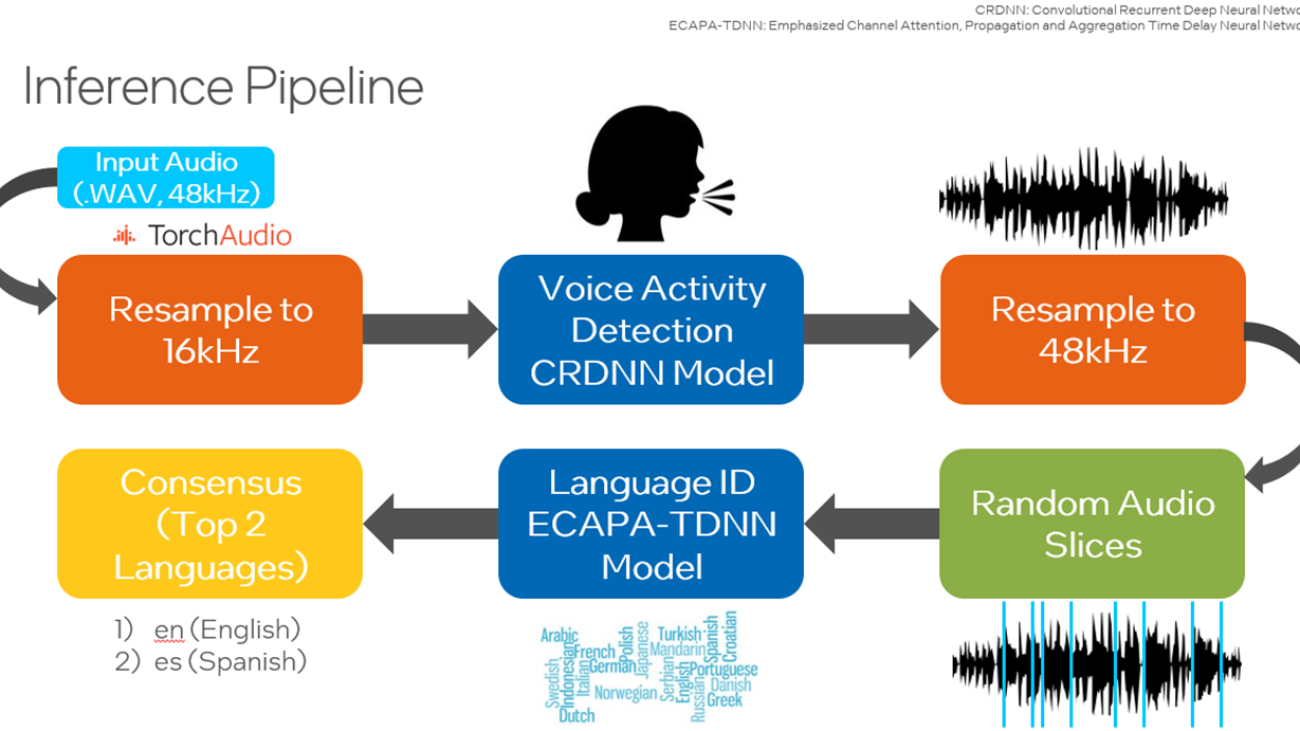
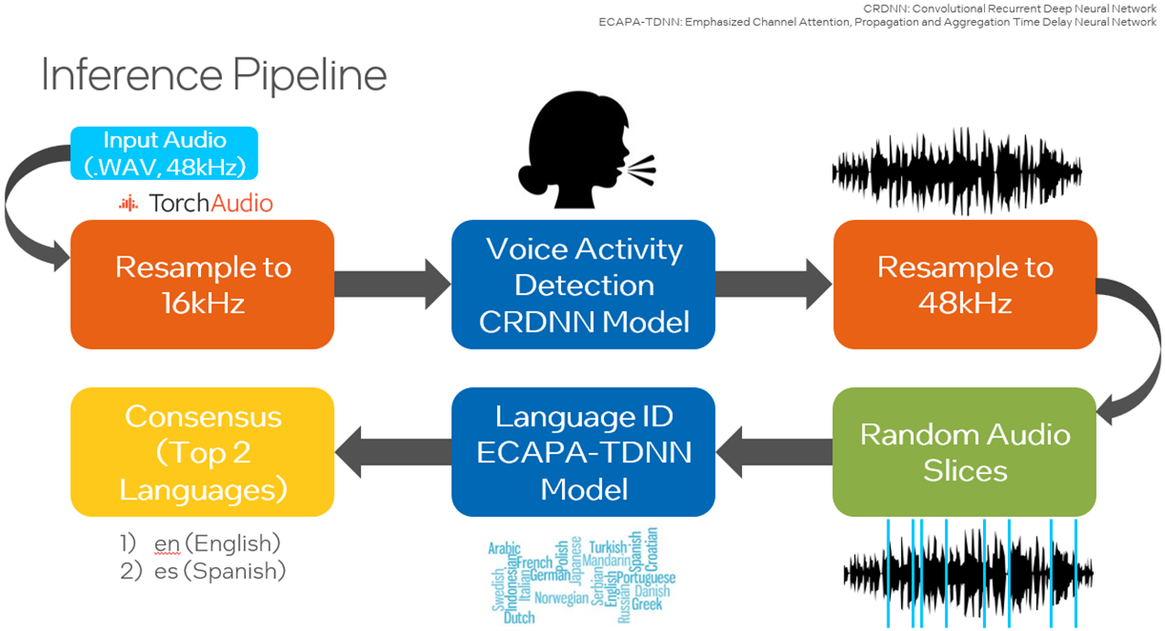
A small Convolutional Recurrent Deep Neural Network (CRDNN) pretrained on the LibriParty dataset is used to process audio samples and output the segments where speech activity is detected. This can be used in inference with the --vad option.
From the figure below, the timestamps where speech will be detected is delivered from the CRDNN model, and these are used to construct a new, shorter audio file with only speech. Sampling from this new audio file will give a better prediction of the primary language spoken.
Run the inference script yourself. An example command of running inference:
python inference_custom.py -p data_custom -d 3 -s 50 --vad
This will run inference on data you provide located inside the data_custom folder. This command performs inference on 50 randomly selected 3-second audio samples with voice activity detection.
If you want to run the code sample for other languages, download Common Voice Corpus 11.0 datasets for other languages.
Optimizations with Intel Extension for PyTorch and Intel Neural Compressor
PyTorch
The Intel extension expands PyTorch with up-to-date features and optimizations for an extra performance boost on Intel hardware. Check out how to install Intel Extension for PyTorch. The extension can be loaded as a Python module or linked as a C++ library. Python users can enable it dynamically by importing intel_extension_for_pytorch.
- The CPU tutorial gives detailed information about Intel Extension for PyTorch for Intel CPUs. Source code is available at the master branch.
- The GPU tutorial gives detailed information about Intel Extension for PyTorch for Intel GPUs. Source code is available at the xpu-master branch.
To optimize the model for inference using Intel Extension for PyTorch, the --ipexoption can be passed in. The model is optimized using the plug-in. TorchScript speeds up inference because PyTorch is run in graph mode. The command to run with this optimization is:
python inference_custom.py -p data_custom -d 3 -s 50 --vad --ipex --verbose
Note: The --verbose option is required to view the latency measurements.
Auto-mixed precision such as bfloat16 (BF16) support will be added in a future release of the code sample.
Intel Neural Compressor
This is an open-source Python library that runs on CPUs or GPUs, which:
- Performs model quantization to reduce the model size and increase the speed of deep learning inference for deployment.
- Automates popular methods such as quantization, compression, pruning, and knowledge distillation across multiple deep-learning frameworks.
- Is part of the AI Kit
The model can be quantized from float32 (FP32) precision to integer-8 (INT8) by running the quantize_model.py script while passing in the path to the model and a validation dataset. The following code can be used to load this INT8 model for inference:
from neural_compressor.utils.pytorch import load
model_int8 = load("./lang_id_commonvoice_model_INT8", self.language_id)
signal = self.language_id.load_audio(data_path)
prediction = self.model_int8(signal)
Note that the original model is required when loading the quantized model. The command to quantize the trained model from FP32 to INT8 by using quantize_model.py is:
python quantize_model.py -p ./lang_id_commonvoice_model -datapath $COMMON_VOICE_PATH/commonVoiceData/commonVoice/dev
What’s Next?
Try out the above code sample by upgrading the hardware to a 4th Generation Intel Xeon Scalable Processor with Intel AMX and identify up to 93 different languages from Common Voice datasets.
We encourage you to learn more about and incorporate Intel’s other AI/ML Framework optimizations and end-to-end portfolio of tools into your AI workflow. Also, visit AI & ML page covering Intel’s AI software development resources for preparing, building, deploying, and scaling your AI solutions.
For more details about the new 4th Gen Intel Xeon Scalable processors, visit Intel’s AI Solution Platform portal where you can learn how Intel is empowering developers to run end-to-end AI pipelines on these powerful CPUs.
Useful resources
- Intel AI Developer Tools and resources
- oneAPI unified programming model
- Official documentation – Intel® Optimization for TensorFlow*
- Official documentation – Intel® Neural Compressor
- Accelerate AI Workloads with Intel® AMX
Explore more AI code samples

American Sign Language Fingerspelling Recognition
 Posted by Thad Starner (Professor, Georgia Tech and Staff Research Scientist, Google), Sam Sepah (ML Research Program Manager), Manfred Georg (Software Engineer, Google), Mark Sherwood (Senior Product Manager, Google), Glenn Cameron (Product Marketing Manager, Google)

Over 70 million deaf people around the world use sign language to communicate. Collectively, they use more than 300 different sign languages worldwide. And over 1.5 billion people are affected by hearing loss globally. Most Deaf and Hard of Hearing people cannot use their voice to initiate a search or perform actions due to speech limitations. Additionally, the interfaces used by smart home devices and mobile platforms to respond to speech are generally audio based.
Signed languages are sophisticated systems of communication, each with a complete set of language features. On a surface level, handshapes along with four other “parameters” form the basis of signed communication. An open hand or a closed hand while making the same motion can completely change the meaning of a sign. Likewise, palm orientation, motion/contact, location, and non-manual markers (typically mouth movements and facial expressions) define individual signs. A number of grammatical constructs, some of which have no analog in spoken languages, allow a signer to produce complex phrases.
As we develop translation systems for American Sign Language (ASL) and other sign languages, it is natural to break apart various aspects of the language and attempt to perform tasks using those parts.
To that end, we’re excited to announce the release of one of the largest datasets of ASL fingerspelling and a Kaggle ML competition that will award $200k in prizes to ML engineers who develop the most accurate ASL fingerspelling recognition models using MediaPipe and TensorFlow Lite. The winning models will be open sourced to help developers add support for fingerspelling to their apps.
| Watch These Hands (Kaggle remix) Performed by Sean Forbes, Co-Founder, Deaf Professional Arts Network |
Fingerspelling communicates words using hand shapes that represent individual letters. While fingerspelling is only a part of sign languages, it is often used for communicating names, addresses, phone numbers, names, and other information that is commonly entered on a mobile phone. Many Deaf smartphone users can fingerspell words faster than they can type on mobile keyboards. In fact, in our dataset, ASL fingerspelling of phrases averages 57 words per minute, which is substantially faster than the US average of 36 words per minute for an on screen keyboard. But, sign language recognition AI for text entry lags far behind voice-to-text or even gesture-based typing, as robust datasets didn’t previously exist.
Although fingerspelling is just a small part of sign languages, there are many reasons to produce systems which specifically focus on it, even while maintaining an ultimate goal of full translation. While fingerspelling at full speed (which can peak over 80 words per minute) the handshapes in the fingerspelling co-articulate together and entire words can become lexicalized into different shapes from their slowed down version. The resulting movements are visually among the fastest used in ASL, and thus stretch particular aspects of any visual recognition system which seeks to perform full translation.
Big Steps Forward
Google Research and the Deaf Professional Arts Network have worked together to create a massive fingerspelling dataset that we will release for this competition to help move sign language recognition forward. The dataset includes over 3 million fingerspelled characters produced by over 100 Deaf signers in the form of continuous phrases, names, addresses, phone numbers, and URLs. This signing was captured using the selfie camera of a smartphone with a variety of backgrounds and lighting conditions and is the largest dataset collection of its kind to date.
Large language models show increasing promise in a variety of language and speech tasks. Everything from chat agents to assistant technology is progressing at breathtaking speed. It is time to ensure that gesture and visual based systems also produce usable interfaces. Fingerspelling recognition models are part of this larger solution, which will address the widening gap in accessibility for Deaf and Hard of Hearing individuals.
How to Get Involved
Join the Kaggle competition today to help us make AI more accessible for the Deaf and hard of hearing community.