Real world images often have highly imbalanced content density. Some areas are very uniform, e.g., large patches of blue sky, while other areas are scattered with many small objects. Yet, the commonly used successive grid downsampling strategy in convolutional deep networks treats all areas equally. Hence, small objects are represented in very few spatial locations, leading to worse results in tasks such as segmentation. Intuitively, retaining more pixels representing small objects during downsampling helps to preserve important information. To achieve this, we propose AutoFocusFormer (AFF), a…Apple Machine Learning Research
Learning to Detect Novel and Fine-Grained Acoustic Sequences Using Pretrained Audio Representations
This work investigates pre-trained audio representations for few shot Sound Event Detection. We specifically address the task of few shot detection of novel acoustic sequences, or sound events with semantically meaningful temporal structure, without assuming access to non-target audio. We develop procedures for pre-training suitable representations, and methods which transfer them to our few shot learning scenario. Our experiments evaluate the general purpose utility of our pre-trained representations on AudioSet, and the utility of proposed few shot methods via tasks constructed from…Apple Machine Learning Research
Amazon-sponsored workshop advances deep learning for code
ICLR workshop sponsored by Amazon CodeWhisperer features Amazon papers on a novel contrastive-learning framework for causal language models and a way to gauge the robustness of code generation models.Read More

Renders and Dragons Rule Creative Kingdoms This Week ‘In the NVIDIA Studio’
Editor’s note: This post is part of our weekly In the NVIDIA Studio series, which celebrates featured artists, offers creative tips and tricks, and demonstrates how NVIDIA Studio technology improves creative workflows. We’re also deep diving on new GeForce RTX 40 Series GPU features, technologies and resources, and how they dramatically accelerate content creation.
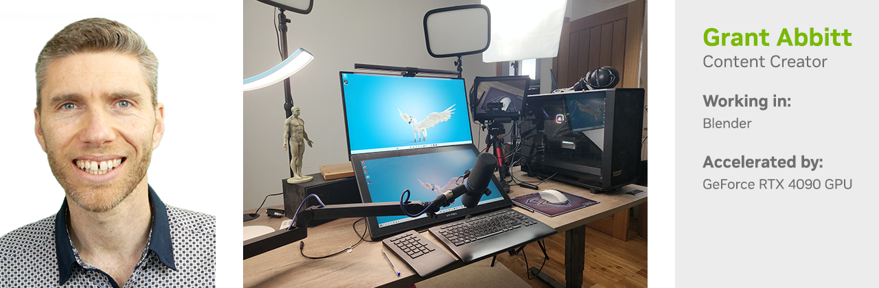
Content creator Grant Abbitt embodies selflessness, one of the best qualities that a creative can possess. Passionate about giving back to the creative community, Abbitt offers inspiration, guidance and free education for others in his field through YouTube tutorials.
He designed Dragon, the 3D scene featured this week In the NVIDIA Studio, specifically to help new Blender users easily understand the steps in the creative process of using the software.
“Dragons can be extremely tough to make,” said Abbitt. While he could have spent more time refining the details, he said, “That wasn’t the point of the project. It’s all about the learning journey for the student.”
Abbitt understands the importance of early education. Providing actionable, straightforward instructions enables prospective 3D modelers to make gradual progress, he said. When encouraged, 3D artists keep morale high while gaining confidence and learning more advanced skills, Abbitt has noticed over his 30+ years of industry experience.
His own early days of learning 3D workflows presented unique obstacles, like software programs costing as much as the hardware, or super-slow internet, which required Abbitt to learn 3D through instructional VHS tapes.

Undeterred by such challenges, Abbitt earned a media studies degree and populated films with his own 3D content.
Now a full-time 3D artist and content creator, Abbitt does what he loves while helping aspiring content creators realize their creative ambitions. In this tutorial, for example, Abbitt teaches viewers how to create a video game character in just 20 minutes.
Dragon Wheel
Abbitt described a different dynasty in this realm — how he created his Dragon piece.
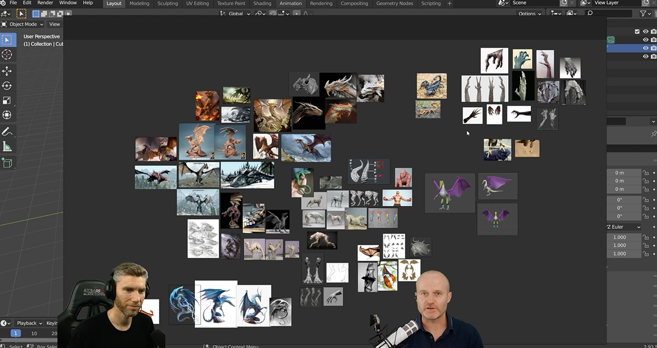
“Reference images are a must,” stressed Abbitt. “Deviation from the intended vision is part of the creative process, but without a direction or foundation, things can quickly go off track.” This is especially important with freelance work and creative briefs provided by clients, he added.
Abbitt looked to Pinterest and ArtStation for creative inspiration and reference material, and sketched in the Krita app on his tablet. The remainder of the project was completed in Blender — the popular 3D creation suite — which is free and open source.
He began with the initial blockout, a 3D rough-draft level built using simple 3D shapes without details or polished art assets. The goal of the blockout was to prototype, test and adjust the foundational shapes of the dragon. Abbitt then combined block shapes into a single mesh model, the structural build of a 3D model, consisting of polygons.
More sculpting was followed by retopologizing the mesh, the process of simplifying the topology of a mesh to make it cleaner and easier to work with. This is a necessary step for images that will undergo more advanced editing and distortions.
Adding Blender’s multiresolution modifier enabled Abbitt to subdivide a mesh, especially useful for re-projecting details from another sculpt with a Shrinkwrap modifier, which allows an object to “shrink” to the surface of another object. It can be applied to meshes, lattices, curves, surfaces and texts.
At this stage, the power of Abbitt’s GeForce RTX 4090 GPU really started to shine. He sculpted fine details faster with Blender Cycles RTX-accelerated OptiX ray tracing in the viewport for fluid, interactive modeling with photorealistic detail. Baking and applying textures were done with buttery smooth ease.
The RTX 4090 GPU also accelerated the animation phase, where the artist rigged and posed his model. “Modern content creators require GPU technology to see their creative visions fully realized at an efficient pace,” Abbitt said.
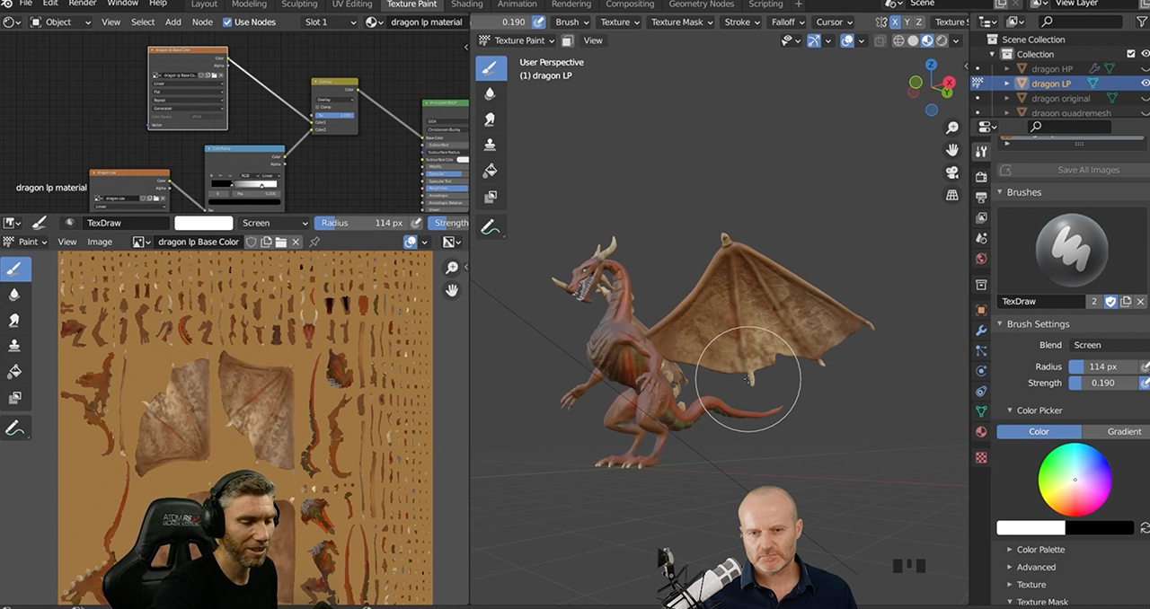
For the texturing, painting and rendering process, Abbitt said he found it “extremely useful to be able to see the finished results without a huge render time, thanks to NVIDIA OptiX.”
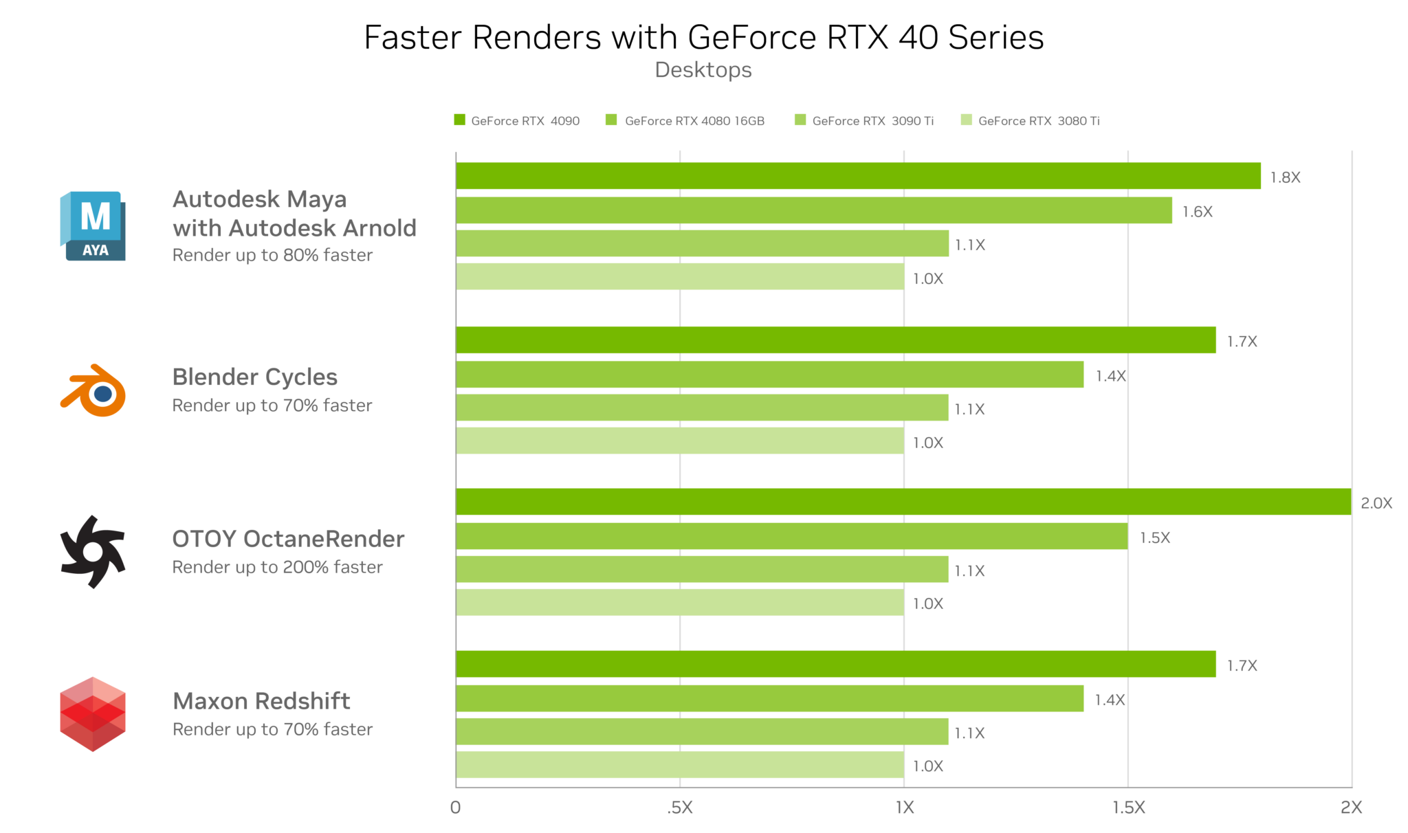
Rendering final files in popular 3D creative apps — like Blender, Autodesk Maya with Autodesk Arnold, OTOY’s OctaneRender and Maxon’s Redshift — is made 70-200% faster with an RTX 4090 GPU, compared to previous-generation cards. This results in invaluable time saved for a freelancer with a deadline or a student working on a group project.
Abbitt’s RTX GPU enabled OptiX ray tracing in Blender Cycles for the fastest final frame render.

“NVIDIA GeForce RTX graphics cards are really the only choice at the moment for Blender users, because they offer so much more speed during render times,” said Abbitt. “You can quickly see results and make the necessary changes.”
Check out Abbitt’s YouTube channel with livestreams every Friday at 9 a.m. PT.
Follow NVIDIA Studio on Instagram, Twitter and Facebook. Access tutorials on the Studio YouTube channel and get updates directly in your inbox by subscribing to the Studio newsletter.

Accelerated Image Segmentation using PyTorch
Using Intel® Extension for PyTorch to Boost Image Processing Performance
PyTorch delivers great CPU performance, and it can be further accelerated with Intel® Extension for PyTorch. I trained an AI image segmentation model using PyTorch 1.13.1 (with ResNet34 + UNet architecture) to identify roads and speed limits from satellite images, all on the 4th Gen Intel® Xeon® Scalable processor.
I will walk you through the steps to work with a satellite image dataset called SpaceNet5 and how I optimized the code to make deep learning workloads feasible on CPUs just by flipping a few key switches.
Before we get started, some housekeeping…
The code accompanying this article is available in the examples folder in the Intel Extension for PyTorch repository. I borrowed heavily from the City-Scale Road Extraction from Satellite Imagery (CRESI) repository. I adapted it for the 4th Gen Intel Xeon processors with PyTorch optimizations and Intel Extension for PyTorch optimizations. In particular, I was able to piece together a workflow using the notebooks here.
You can find the accompanying talk I gave on YouTube.
I also highly recommend these articles for a detailed explanation of how to get started with the SpaceNet5 data:
- The SpaceNet 5 Baseline — Part 1: Imagery and Label Preparation
- The SpaceNet 5 Baseline — Part 2: Training a Road Speed Segmentation Model
- The SpaceNet 5 Baseline — Part 3: Extracting Road Speed Vectors from Satellite Imagery
- SpaceNet 5 Winning Model Release: End of the Road
I referenced two Hugging Face blogs by Julien Simon; he ran his tests on the AWS instance r7iz.metal-16xl:
- Accelerating PyTorch Transformers with Intel Sapphire Rapids, part 1
- Accelerating PyTorch Transformers with Intel Sapphire Rapids, part 2
The potential cost savings from using a CPU instance instead of a GPU instance on the major cloud service providers (CSP) can be significant. The latest processors are still being rolled out to the CSPs, so I’m using a 4th Gen Intel Xeon processor that is hosted on the Intel® Developer Cloud (you can sign up for the Beta here: cloud.intel.com).
On AWS, you can select from the r7iz.* EC2 instances after you sign up for the preview here (Figure 1). At the time of writing, the new AI-acceleration engine, Intel® Advanced Matrix Extensions (Intel® AMX), is only available on bare metal but it should soon be enabled on the virtual machines.
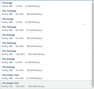
Figure 1. List of 4th Gen Xeon instances on AWS EC2 (image by author)
On Google Cloud* Platform, you can select from the 4th Gen Xeon Scalable processors C3 VMs (Figure 2).
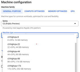
Figure 2. List of 4th Gen Intel Xeon Scalable processor instances on Google Cloud Platform (image by author)
Hardware Introduction and Optimizations
The 4th Gen Intel Xeon processors were released January 2023, and the bare-metal instance I am using has two sockets (each with 56 physical cores), 504 GB of memory, and Intel AMX acceleration. I installed a few key libraries in the backend to take control and monitor the sockets, memory, and cores that I am using on the CPU:
numactl (with sudo apt-get install numactl)
libjemalloc-dev (with sudo apt-get install libjemalloc)
intel-openmp (with conda install intel-openmp)
gperftools (with conda install gperftools -c conda-forge)
Both PyTorch and Intel Extension for PyTorch have helper scripts so that one does not need to explicitly use intel-openmp and numactl, but they do need to be installed in the backend. In case you want to set them up for other work, here is what I used for OpenMP* …
export OMP_NUM_THREADS=36
export KMP_AFFINITY=granularity=fine,compact,1,0
export KMP_BLOCKTIME=1
… where OMP_NUM_THREADS is the number of threads allocated to the job, KMP_AFFINITY affects thread affinity settings (including packing threads close to each other, the state of pinning threads), and KMP_BLOCKTIME sets the time in milliseconds that an idle thread should wait before going to sleep.
Here’s what I used for numactl …
numactl -C 0-35 --membind=0 train.py
…where -C specifies which cores to use and --membind instructs the program to only use one socket (socket 0 in this case).
SpaceNet Data
I am using a satellite image dataset from the SpaceNet 5 Challenge. Different cities can be downloaded for free from an AWS S3 bucket:
aws s3 ls s3://spacenet-dataset/spacenet/SN5_roads/tarballs/ --human-readable
2019-09-03 20:59:32    5.8 GiB SN5_roads_test_public_AOI_7_Moscow.tar.gz
2019-09-24 08:43:02    3.2 GiB SN5_roads_test_public_AOI_8_Mumbai.tar.gz
2019-09-24 08:43:47    4.9 GiB SN5_roads_test_public_AOI_9_San_Juan.tar.gz
2019-09-14 13:13:26   35.0 GiB SN5_roads_train_AOI_7_Moscow.tar.gz
2019-09-14 13:13:34   18.5 GiB SN5_roads_train_AOI_8_Mumbai.tar.gz
You can use the following commands to download and unpack a file:
aws s3 cp s3://spacenet-dataset/spacenet/SN5_roads/tarballs/SN5_roads_train_AOI_7_Moscow.tar.gz .
tar -xvzf ~/spacenet5data/moscow/SN5_roads_train_AOI_7_Moscow.tar.gz
Dataset Preparation
I used the Moscow satellite image dataset, which consists of 1,352 images of 1,300 by 1,300 pixels with corresponding street labels in separate text files. The dataset contains both 8-band multispectral images and 3-band RGB images. Figure 3 shows four sample RGB satellite images and their corresponding generated masks. I used the speed_masks.py script from the CRESI repository to generate the segmentation masks.
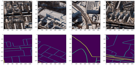
Figure 3. Satellite image 3-channel RGB chips from Moscow (top row) and corresponding pixel segmentation masks with varying speed limits (bottom row) (image by author)
There is a JSON configuration file that must be updated for all remaining components: training and validation split, training, and inference. An example configuration can be found here. I perform an 80:20 training/validation split, making sure to point to the correct folder of satellite images and corresponding masks for training. The configuration parameters are explained in more in the notebook under examples in GitHub for Intel Extension for PyTorch here.
Training a ResNet34 + UNet Model
I made some changes to the cresi code described below in order to run on a CPU and optimize the training. To run natively on a CPU, replace self.model = nn.DataParallel(model).cuda() with self.model = nn.DataParallel(model) in the train.py script. In the 01_train.py script, remove torch.randn(10).cuda().
To optimize training, add import intel_extension_for_pytorch as ipex to the import statements in the train.py script. Just after defining the model and optimizer as follows:
self.model = nn.DataParallel(model)
self.optimizer = optimizer(self.model.parameters(), lr=config.lr)
Add the ipex.optimize line to use BF16 precision, instead of FP32:
self.model, self.optimizer = ipex.optimize(self.model,
    optimizer=self.optimizer,dtype=torch.bfloat16)
Add a line to do mixed-precision training just before running a forward pass and calculating the loss function:
with torch.cpu.amp.autocast():
    if verbose:
        print("input.shape, target.shape:", input.shape, target.shape)
    output = self.model(input)
    meter = self.calculate_loss_single_channel(output, target, meter, training, iter_size)
Now that we have optimized our training code, we can move onto training our model.
Like the winner of the SpaceNet 5 competition, I trained a ResNet34 encoder + UNet decoder model. It is pretrained from ImageNet weights, and the backbone is left completely unfrozen during training. The training can be run with the 01_train.py script, but in order to control the use of hardware I used a helper script. There are actually two helper scripts: one that comes with stock PyTorch and one that comes with Intel Extension for PyTorch. They both accomplish the same thing, but the first one from stock is torch.backends.xeon.run_cpu, and the second one from Intel Extension for PyTorch is ipexrun.
Here is what I ran in the command-line:
python -m torch.backends.xeon.run_cpu --ninstances 1
  --ncores_per_instance 32
  --log_path /home/devcloud/spacenet5data/moscow/v10_xeon4_devcloud22.04/logs/run_cpu_logs
  /home/devcloud/cresi/cresi/01_train.py
  /home/devcloud/cresi/cresi/configs/ben/v10_xeon4_baseline_ben.json --fold=0
ipexrun --ninstances 1
--ncore_per_instance 32
/home/devcloud/cresi/cresi/01_train.py
/home/devcloud/cresi/cresi/configs/ben/v10_xeon4_baseline_ben.json --fold=0
In both cases, I am asking PyTorch to run training on one socket with 32 cores. Upon running, I get a printout of what environment variables get set in the backend to understand how PyTorch is using the hardware:
INFO - Use TCMalloc memory allocator
INFO - OMP_NUM_THREADS=32
INFO - Using Intel OpenMP
INFO - KMP_AFFINITY=granularity=fine,compact,1,0
INFO - KMP_BLOCKTIME=1
INFO - LD_PRELOAD=/home/devcloud/.conda/envs/py39/lib/libiomp5.so:/home/devcloud/.conda/envs/py39/lib/libtcmalloc.so
INFO - numactl -C 0-31 -m 0 /home/devcloud/.conda/envs/py39/bin/python -u 01_train.py configs/ben/v10_xeon4_baseline_ben.json --fold=0
During training, I make sure that my total loss function is decreasing (i.e., the model is converging on a solution).
Inference
After training a model, we can start to make predictions from satellite images alone. In the eval.py inference script, add import intel_extension_for_pytorch as ipex to the import statements. After loading the PyTorch model, use Intel Extension for PyTorch to optimize the model for BF16 inference:
model = torch.load(os.path.join(path_model_weights,
    'fold{}_best.pth'.format(fold)),
    map_location = lambda storage,
    loc: storage)
model.eval()
model = ipex.optimize(model, dtype = torch.bfloat16)
Just prior to running prediction, add two lines for mixed precision:
with torch.no_grad():
    with torch.cpu.amp.autocast():
        for data in pbar:
            samples = torch.autograd.Variable(data['image'], volatile=True)
            predicted = predict(model, samples, flips=self.flips)
To run inference, we can use the 02_eval.py script. Now that we have a trained model, we can make predictions on satellite images (Figure 4). We can see that it does seem to map the roads closely to the image!
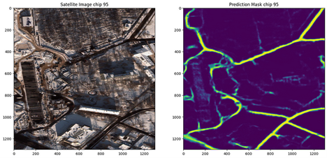
Figure 4. Moscow satellite image and accompanying prediction of roads (image by author)
I realize that the model I’ve trained is overfit to the Moscow image data and probably won’t generalize well to other cities. However, the winning solution to this challenge used data from six cities (Las Vegas, Paris, Shanghai, Khartoum, Moscow, Mumbai) and performs well on new cities. In the future, one thing that would be worth testing is training on all six cities and running inference on another city to reproduce their results.
Note on Post-Processing
There are further post-processing steps that can be performed to add the mask as graph features to maps. You can read more about the post-processing steps here:
The SpaceNet 5 Baseline — Part 3: Extracting Road Speed Vectors from Satellite Imagery
Conclusions
In summary, we:
- Created 1,352 image training masks (with speed limits) to correspond to our training satellite image data (from .geojson text file labels)
- Defined our configuration file for training and inference
- Split up our data into training and validation sets
- Optimized our code for CPU training, including using Intel Extension for PyTorch and BF16
- Trained a performant ResNet34 + UNet model on a 4th Gen Intel Xeon CPU
- Ran initial inference to see the prediction of a speed limit mask
You can find detailed benchmarks here for the 4th Gen Intel Xeon CPU here.
Next Steps
Extend the optimizations on an Intel CPU by using the Intel Extension for PyTorch:
pip install intel-extension-for-pytorch
git clone https://github.com/intel/intel-extension-for-pytorch
Get in touch with me on LinkedIn if you have any more questions!
More information about the Intel Extension for PyTorch can be found here.
Get the Software
I encourage you to check out Intel’s other AI Tools and Framework optimizations and learn about the open, standards-based oneAPI multiarchitecture, multivendor programming model that forms the foundation of Intel’s AI software portfolio.
For more details about 4th Gen Intel Xeon Scalable processor, visit AI Platform where you can learn about how Intel is empowering developers to run high-performance, efficient end-to-end AI pipelines.
PyTorch Resources
Prepare image data with Amazon SageMaker Data Wrangler
The rapid adoption of smart phones and other mobile platforms has generated an enormous amount of image data. According to Gartner, unstructured data now represents 80–90% of all new enterprise data, but just 18% of organizations are taking advantage of this data. This is mainly due to a lack of expertise and the large amount of time and effort that’s required to sift through all that information to identify quality data and useful insights.
Before you can use image data for labeling, training, or inference, it first needs to be cleaned (deduplicate, drop corrupted images or outliers, and so on), analyzed (such as group images based on certain attributes), standardized (resize, change orientation, standardize lighting and color, and so on), and augmented for better labeling, training, or inference results (enhance contrast, blur some irrelevant objects, upscale, and so on).
Today, we are happy to announce that with Amazon SageMaker Data Wrangler, you can perform image data preparation for machine learning (ML) using little to no code.
Data Wrangler reduces the time it takes to aggregate and prepare data for ML from weeks to minutes. With Data Wrangler, you can simplify the process of data preparation and feature engineering, and complete each step of the data preparation workflow (including data selection, cleansing, exploration, visualization, and processing at scale) from a single visual interface.
Data Wrangler’s image data preparation feature addresses your needs via a visual UI for image preview, import, transformation, and export. You can browse, import, and transform image data just like how you use Data Wrangler for tabular data. In this post, we show an example of how to use this feature.
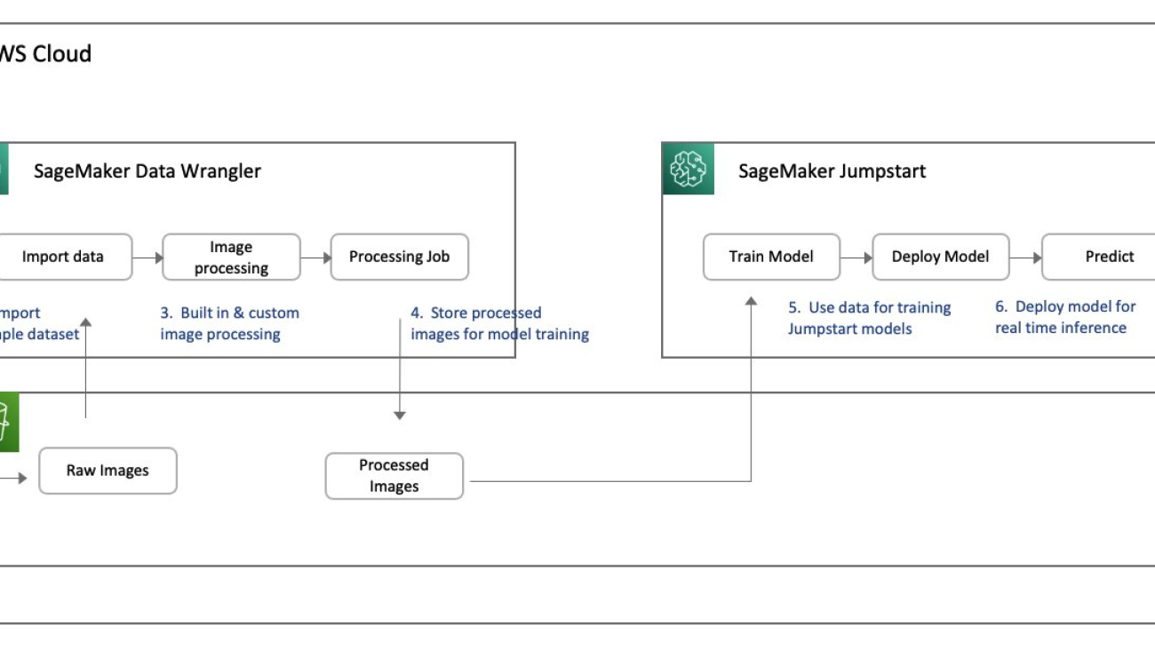
Solution overview
For this post, we focus on the Data Wrangler component of image processing, which we use to help an image classification model detect crashes with better quality images. We use the following services:
- Amazon SageMaker Data Wrangler to perform image processing
- Amazon SageMaker Jumpstart to train a image recognition model using the prepared dataset
- Amazon SageMaker Studio notebooks to test the model
The following diagram illustrates the solution architecture.

Data Wrangler is a SageMaker feature available within Studio. You can follow the Studio onboarding process to spin up the Studio environment and notebooks. Although you can choose from a few authentication methods, the simplest way to create a Studio domain is to follow the Quick start instructions. The Quick start uses the same default settings as the standard Studio setup. You can also choose to onboard using AWS IAM Identity Center (successor to AWS Single Sign-On) for authentication (see Onboard to Amazon SageMaker Domain Using IAM Identity Center).
For this use case, we use CCTV footage data of accidents and non-accidents available from Kaggle. The dataset contains frames captured from YouTube videos of accidents and non-accidents. The images are split into train, test, and validation folders.
Prerequisites
As a prerequisite, download the sample dataset and upload it to an Amazon Simple Storage Service (Amazon S3) bucket. We use this dataset for image processing and subsequently for training a custom model.
Process images using Data Wrangler
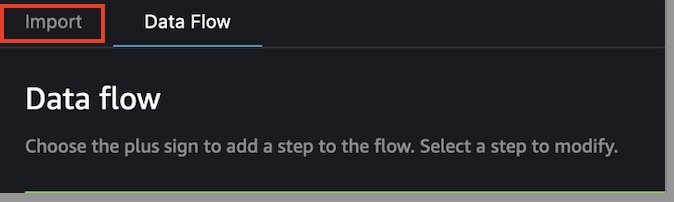
Start your Studio environment and create a new Data Wrangler flow called car_crash_detection_data.flow. Now let’s import the dataset to Data Wrangler from the S3 bucket where the dataset was uploaded. Data Wrangler allows you to import datasets from different data sources, including images.
Data Wrangler supports a variety of built-in transformations for image processing, including the following:
- Blur image – Data Wrangler supports different techniques from an open-source image library (Gaussian, Average, Median, Motion, and more) for blurring images. For details of each technique, refer to augmenters.blur.
- Corrupt image – Data Wrangler also supports different corruption techniques (Gaussian noise, Impulse noise, Speckle noise, and more). For details of each technique, refer to augmenters.imgcorruptlike.
- Enhance image contrast – You can deploy different contrast enhancement techniques (Gamma contrast, Sigmoid contrast, Log contrast, Linear contrast, Histogram equalization, and more). For more details, refer to augmenters.contrast.
- Resize image – Data Wrangler supports different resizing techniques (cropping, padding, thumbnail, and more). For more details, refer to augmenters.size.
In this post, we highlight a subset of these functionalities through the following steps:
- Upload images from the source S3 bucket and preview the image.
- Create quick image transformations using the built-in transformers.
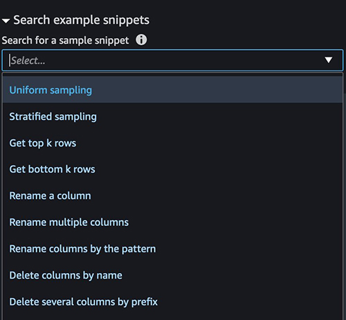
- Write custom code like finding outliers or using the Search Example Snippets function.
- Export the final cleansed data to another S3 bucket.
- Combine images from different Amazon S3 sources into one Data Wrangler flow.
- Create a job to trigger the Data Wrangler flow.
Let’s look at each step in detail.
Upload images from the source bucket S3 and preview the image
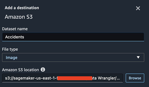
To upload all the images under one folder, complete the following steps:
- Select the S3 folder containing the images.
- For File type, choose Image.
- Select Import nested directories.
- Choose Import.

You can preview the images that you’re uploading by turning the Preview option on. Note that Date Wrangler only imports 100 random images for the interactive data preparation.
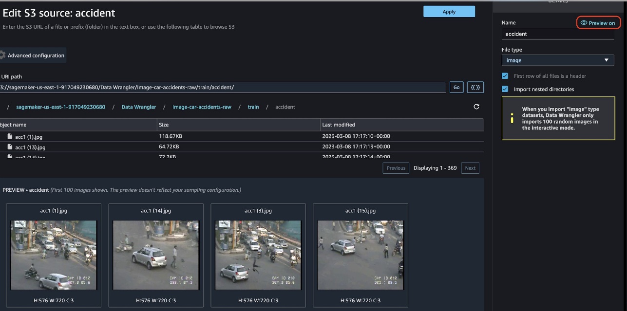
The preview function allows you to view images and preview the quality of images imported.

For this post, we load the images from both the accident and non-accident folders. We create a set of transformations for each: one flow to corrupt images, resize, and remove outliers, and another flow to enhance image contrast, resize, and remove outliers.
Transform images using built-in transformations
Image data transformation is very important to regularize your model network and increase the size of your training set. These transformations can change the images’ pixel values but still keep almost all the information of the image, so that a human could hardly tell whether it was augmented or not. This forces the model to be more flexible with the wide variety of objects in the image, regarding position, orientation, size, color, and so on. Models trained with data augmentation usually generalize better.
Data Wrangler offers you built-in and custom transformations to improve the quality of images for labeling, training, or inference. We use some of these transformations to improve the image dataset fed to the model for machine learning.
Corrupt images
The first built-in transformation we use is Corrupt images.
We add a step with Corruption set to Impulse noise and set our severity.
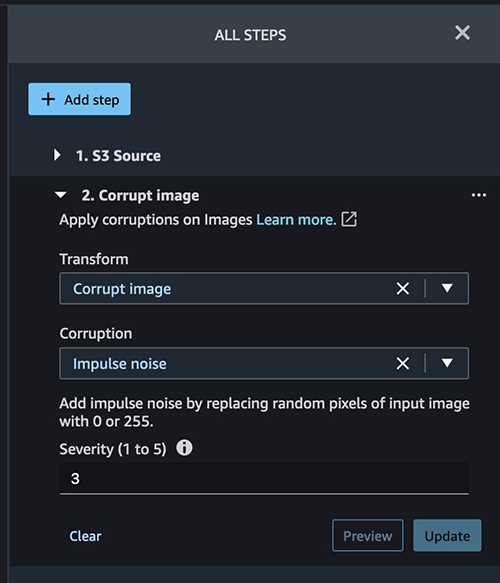
Corrupting an image or creating any kind of noise helps make a model more robust. The model can predict with more accuracy even if it receives a corrupted image because it was trained with corrupt and non-corrupt images.
Enhance contrast
We also add a transform to enhance the Gamma contrast.

Resize images
We can use a built-in transformation to resize all the images to add symmetry. Data Wrangler offers several resize options, as shown in the following screenshot.
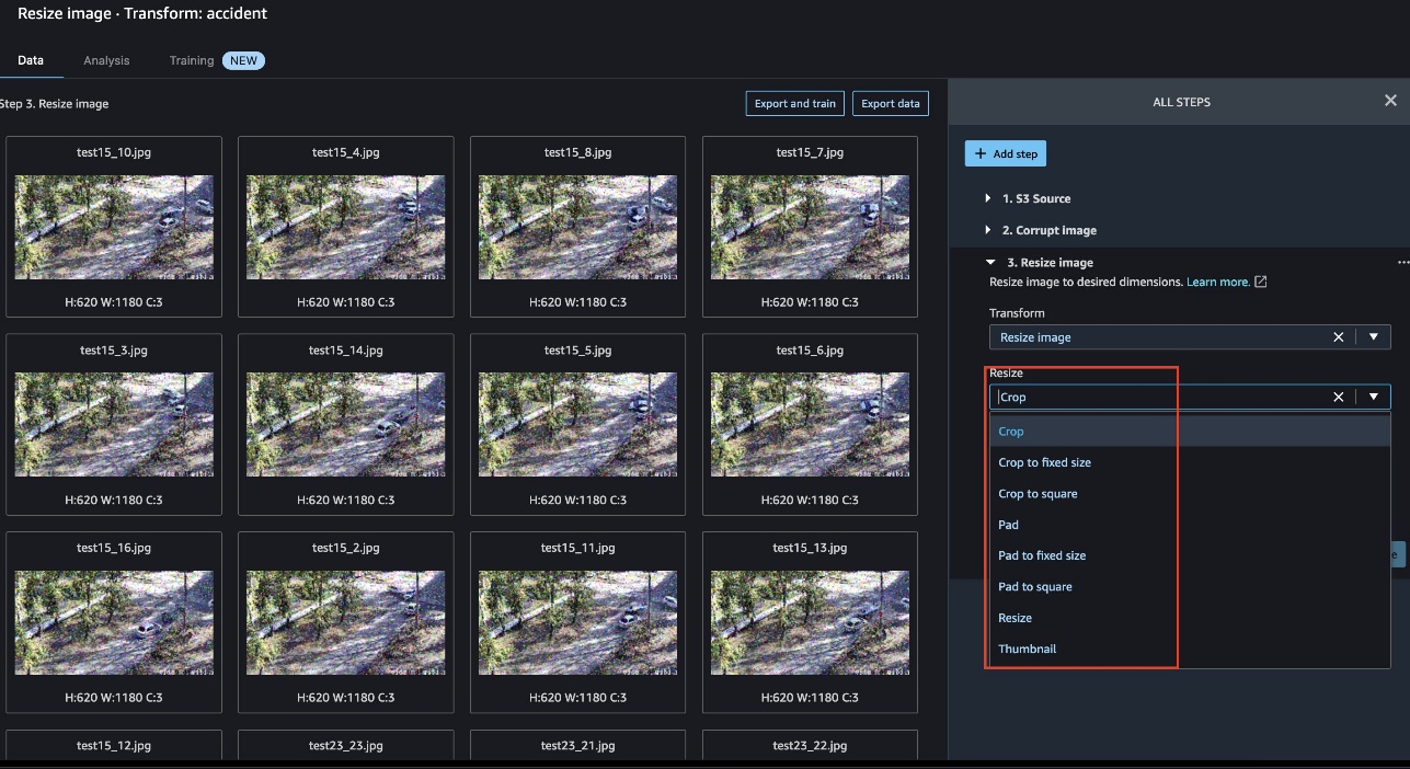
The following example shows images prior to resize: 720 x 1280.

The following images have been resized to 620 x 1180.

Add a custom transformation to detect and remove image outliers
With image preparation in Data Wrangler, we can also invoke another endpoint for another model. You can find some sample scripts with boilerplate code in the Search example snippets section.
For our example, we create a new transformation to remove outliers. Please note that this code is just for demonstration purpose. You may need to modify code to suit any production workload needs.
This is a custom snippet written in PySpark. Before running this step, we need to have an image embedding model mobile-net (for example, jumpstart-dft-mobilenet-v2-100-224-featurevector-4). After the endpoint is deployed, we can call a JumpStart model endpoint.
JumpStart models solve common ML tasks such as image classification, object detection, text classification, sentence pair classification, and question answering, and are available for quick model creation and deployment.
To learn how to create an image embedding model in JumpStart, refer to the GitHub repo. The steps to follow are similar to creating an image classification model with Jumpstart. See the following code:
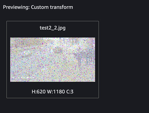
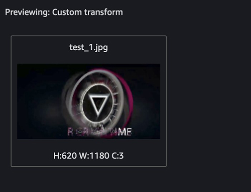
The following screenshots show an example of our custom transform.
This identifies the outlier. Next, let’s filter out the outlier. You can use the following snippet in the end of the custom transform:
Choose Preview and Add to save the changes.
Export the final cleansed data to another S3 bucket
After adding all the transformations, let’s define the destination in Amazon S3.
Provide the location of your S3 bucket.
Combine images from different Amazon S3 sources into one Data Wrangler flow
In the previous sections, we processed images of accidents. We can implement a similar flow for any other images (in our case, non-accident images). Choose Import and follow the same steps to create a second flow.
Now we can view the flows for each dataset.

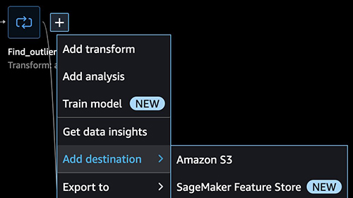
Create a job to run the automated flow
When we create a job, we scale the recipe to the entire dataset, which could be thousands or millions of images. You can also schedule the flow to run periodically, and you can parameterize the input data source to scale the processing. For details on job scheduling and input parameterization, refer to Create a Schedule to Automatically Process New Data.
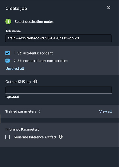
Choose Create job to run a job for the end-to-end flow.

Provide the details of the job and select both datasets.
Congratulations! You have successfully created a job to process images using Data Wrangler.
Model training and deployment
JumpStart provides one-click, end-to-end solutions for many common ML use cases. We can use the images prepared with Data Wrangler when creating a quick image classification model in JumpStart. For instructions, refer to Run image classification with Amazon SageMaker JumpStart.
Clean up
When you’re not using Data Wrangler, it’s important to shut down the instance on which it runs to avoid incurring additional fees.
Data Wrangler automatically saves your data flow every 60 seconds. To avoid losing work, save your data flow before shutting Data Wrangler down.
- To save your data flow in Studio, choose File, then choose Save Data Wrangler Flow.
- To shut down the Data Wrangler instance, in Studio, choose Running Instances and Kernels.
- Under RUNNING APPS, choose the shutdown icon next to the
sagemaker-data-wrangler-1.0app. - Choose Shut down all to confirm.
Data Wrangler runs on an ml.m5.4xlarge instance. This instance disappears from RUNNING INSTANCES when you shut down the Data Wrangler app.
- Shut down the JumpStart endpoint that you created for the outlier transformation image embedding.
After you shut down the Data Wrangler app, it has to restart the next time you open a Data Wrangler flow file. This can take a few minutes.
Conclusion
In this post, we demonstrated using image data preparation for ML on Data Wrangler. To get started with Data Wrangler, see Prepare ML Data with Amazon SageMaker Data Wrangler, and check out the latest information on the Data Wrangler product page.
About the Authors
 Deepmala Agarwal works as an AWS Data Specialist Solutions Architect. She is passionate about helping customers build out scalable, distributed, and data-driven solutions on AWS. When not at work, Deepmala likes spending time with family, walking, listening to music, watching movies, and cooking!
 Meenakshisundaram Thandavarayan works for AWS as an AI/ ML Specialist. He has a passion to design, create, and promote human-centered data and analytics experiences. Meena focusses on developing sustainable systems that deliver measurable, competitive advantages for strategic customers of AWS. Meena is a connector, design thinker, and strives to drive business to new ways of working through innovation, incubation and democratization.
 Lu Huang is a Senior Product Manager on Data Wrangler. She’s passionate about AI, machine learning, and big data.
 Nikita Ivkin is a Senior Applied Scientist at Amazon SageMaker Data Wrangler with interests in machine learning and data cleaning algorithms.

Scaling deep retrieval with TensorFlow Recommenders and Vertex AI Matching Engine
Posted by Jeremy Wortz, ML specialist, Google Cloud & Jordan Totten, Machine Learning Specialist
Cross posted from Google Cloud AI & Machine Learning
In a previous blog, we outlined three approaches for implementing recommendation systems on Google Cloud, including (1) a fully managed solution with Recommendations AI, (2) matrix factorization from BigQuery ML, and (3) custom deep retrieval techniques using two-tower encoders and Vertex AI Matching Engine. In this blog, we dive deep into option (3) and demonstrate how to build a playlist recommendation system by implementing an end-to-end candidate retrieval workflow from scratch with Vertex AI. Specifically, we will cover:
- The evolution of retrieval modeling and why two-tower encoders are popular for deep retrieval tasks
- Framing a playlist-continuation use-case using the Spotify Million Playlist Dataset (MPD)
- Developing custom two-tower encoders with the TensorFlow Recommenders (TFRS) library
- Serving candidate embeddings in an approximate nearest neighbors (ANN) index with Vertex AI Matching Engine
All related code can be found in this GitHub repository.
Background
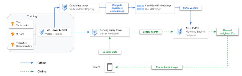
To meet low latency serving requirements, large-scale recommenders are often deployed to production as multi-stage systems. The goal of the first stage (candidate retrieval) is to sift through a large (>100M elements) corpus of candidate items and retrieve a relevant subset (~hundreds) of items for downstream ranking and filtering tasks. To optimize this retrieval task, we consider two core objectives:
- During model training, find the best way to compile all knowledge into
query, candidateembeddings. - During model serving, retrieve relevant items fast enough to meet latency requirements
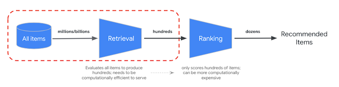 |
| Figure 1: Conceptual components of multi-stage recommendation systems; the focus of this blog is the first stage, candidate retrieval. |
Two-tower architectures are popular for retrieval tasks because they capture the semantics of query and candidate entities, and map these to a shared embedding space such that semantically similar entities cluster closer together. This means, if we compute the vector embeddings of a given query, we can search the embedding space for the closest (most similar) candidates. Because these neural network-based retrieval models take advantage of metadata, context, and feature interactions, they can produce highly informative embeddings and offer flexibility to adjust for various business objectives.
 |
| Figure 2: The two-tower encoder model is a specific type of embedding-based search where one deep neural network tower produces the query embedding and a second tower computes the candidate embedding. Calculating the dot product between the two embedding vectors determines how close (similar) the candidate is to the query. Source: Announcing ScaNN: Efficient Vector Similarity Search. |
While these capabilities help achieve useful query, candidate embeddings, we still need to resolve the retrieval latency requirements. To this end, the two-tower architecture offers one more advantage: the ability to decouple inference of query and candidate items. This decoupling means all candidate item embeddings can be precomputed, reducing the serving computation to (1) converting queries to embedding vectors and (2) searching for similar vectors (among the precomputed candidates).
As candidate datasets scale to millions (or billions) of vectors, the similarity search often becomes a computational bottleneck for model serving. Relaxing the search to approximate distance calculations can lead to significant latency improvements, but we need to minimize negatively impacting search accuracy (i.e., relevance, recall).
In the paper Accelerating Large-Scale Inference with Anisotropic Vector Quantization, Google Researchers address this speed-accuracy tradeoff with a novel compression algorithm that, compared to previous state-of-the-art methods, improves both the relevance and speed of retrieval. At Google, this technique is widely-adopted to support deep retrieval use cases across Search, YouTube, Ads, Lens, and others. And while it’s available in an open-sourced library (ScaNN), it can still be challenging to implement, tune, and scale. To help teams take advantage of this technology without the operational overhead, Google Cloud offers these capabilities (and more) as a managed service with Vertex AI Matching Engine.
The goal of this post is to demonstrate how to implement these deep retrieval techniques using Vertex AI and discuss the decisions and trade-offs teams will need to evaluate for their use cases.
 |
| Figure 3: Figure 3: A reference architecture for two-tower training and deployment on Vertex AI. |
Two-towers for deep retrieval
To better understand the benefits of two-tower architectures, let’s review three key modeling milestones in candidate retrieval.
Evolution of retrieval modeling
Traditional information retrieval systems rely heavily on token-based matching, where candidates are retrieved using an inverted index of n-grams. These systems are interpretable, easy to maintain (e.g., no training data), and are capable of achieving high precision. However, they typically suffer poor recall (i.e., trouble finding all relevant candidates for a given query) because they look for candidates having exact matches of key words. While they are still used for select Search use cases, many retrieval tasks today are either adapted with or replaced by embedding-based techniques.
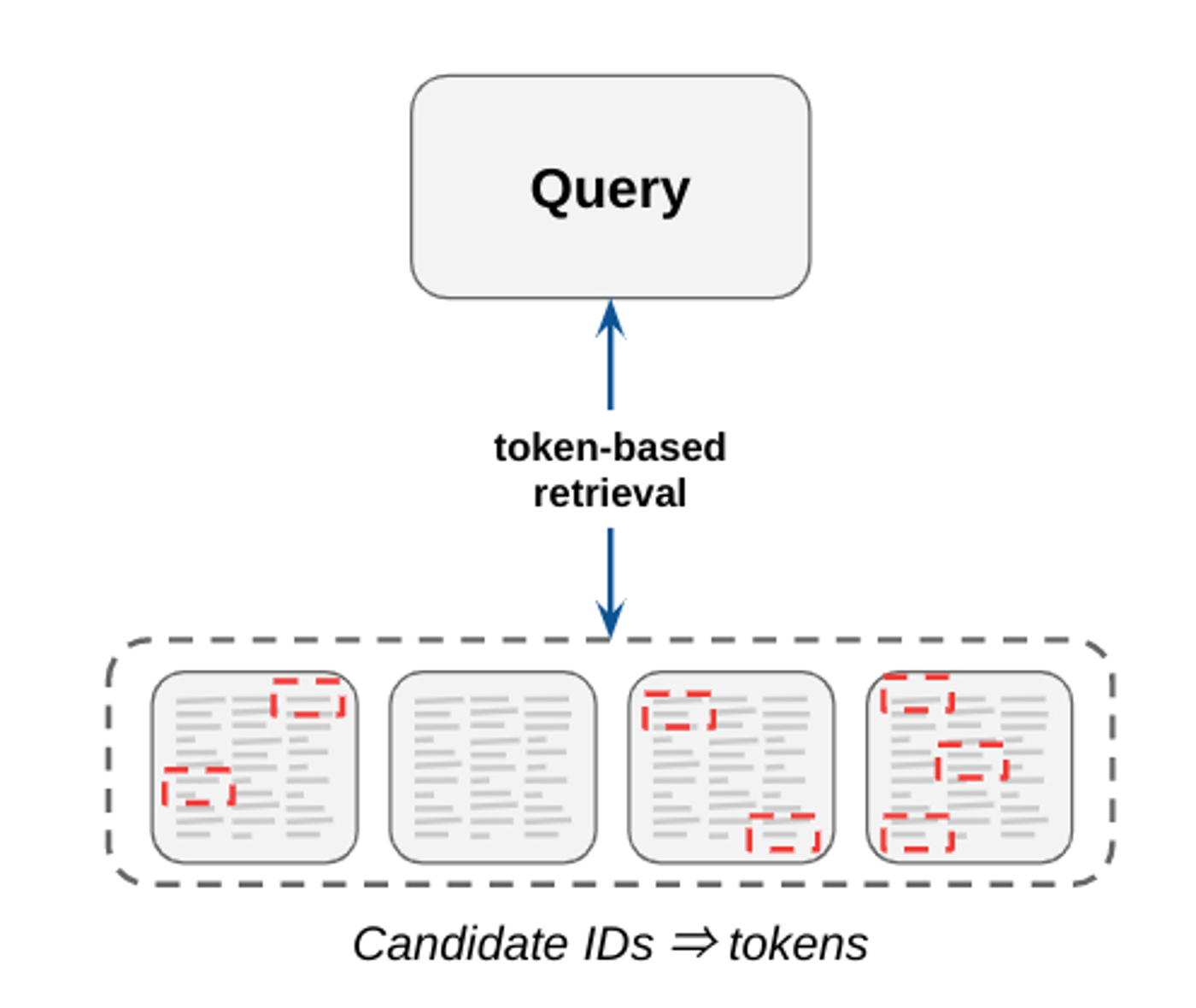 |
| Figure 4: Token-based matching selects candidate items by matching key words found in both query and candidate items. |
Factorization-based retrieval introduces a simple embedding-based model that offers much better generalization by capturing the similarity between query, candidate pairs and mapping them to a shared embedding space. One of the major benefits to this collaborative filtering technique is that embeddings are learned automatically from implicit query-candidate interactions. Fundamentally, these models factorize the full query-candidate interaction (co-occurrence) matrix to produce smaller, dense embedding representations of queries and candidates, where the product of these embedding vectors is a good approximation of the interaction matrix. The idea is that by compacting the full matrix into k dimensions the model learns the top k latent factors describing query, candidate pairs with respect to the modeling task.
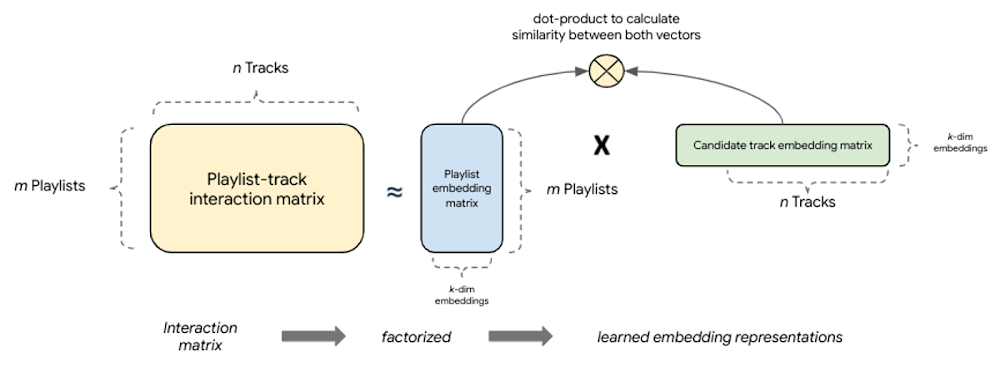 |
| Figure 5: Factorization-based models factorize a query-candidate interaction matrix into the product of two lower-rank matrices that capture the query-candidate interactions. |
The latest modeling paradigm for retrieval, commonly referred to as neural deep retrieval (NDR), produces the same embedding representations, but uses deep learning to create them. NDR models like two-tower encoders apply deep learning by processing input features with successive network layers to learn layered representations of the data. Effectively, this results in a neural network that acts as an information distillation pipeline, where raw, multi-modal features are repeatedly transformed such that useful information is magnified and irrelevant information is filtered. This results in a highly expressive model capable of learning non-linear relationships and more complex feature interactions.
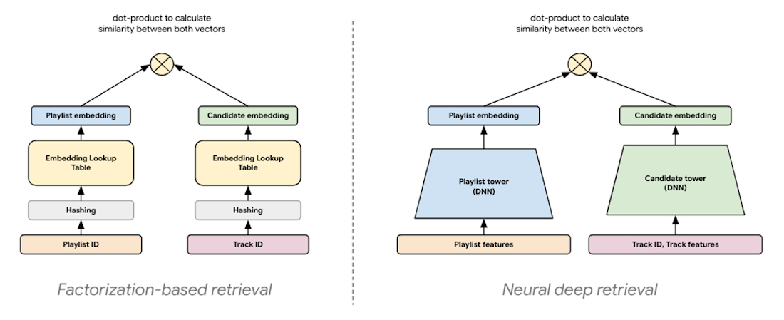 |
| Figure 6: NDR architectures like two-tower encoders are conceptually similar to factorization models. Both are embedding-based retrieval techniques computing lower-dimensional vector representations of query and candidates, where the similarity between these two vectors is determined by computing their dot product. |
In a two-tower architecture, each tower is a neural network that processes either query or candidate input features to produce an embedding representation of those features. Because the embedding representations are simply vectors of the same length, we can compute the dot product between these two vectors to determine how close they are. This means the orientation of the embedding space is determined by the dot product of each query, candidate pair in the training examples.
Decoupled inference for optimal serving
In addition to increased expressivity and generalization, this kind of architecture offers optimization opportunities for serving. Because each tower only uses its respective input features to produce a vector, the trained towers can be operationalized separately. Decoupling inference of the towers for retrieval means we can precompute what we want to find when we encounter its pair in the wild. It also means we can optimize each inference task differently:
- Run a batch prediction job with a trained candidate tower to precompute embedding vectors for all candidates, attach NVIDIA GPU to accelerate computation
- Compress precomputed candidate embeddings to an ANN index optimized for low-latency retrieval; deploy index to an endpoint for serving
- Deploy trained query tower to an endpoint for converting queries to embeddings in real time, attach NVIDIA GPU to accelerate computation
Training two-tower models and serving them with an ANN index is different from training and serving traditional machine learning (ML) models. To make this clear, let’s review the key steps to operationalize this technique.
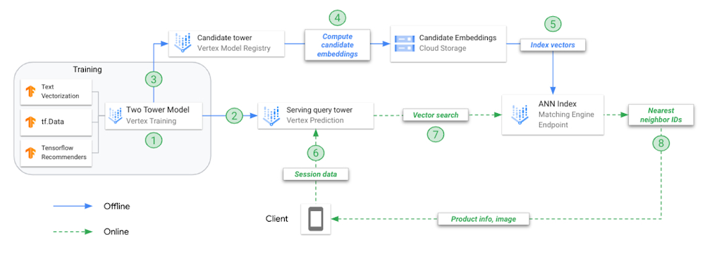 |
| Figure 7: A reference architecture for two-tower training and deployment on Vertex AI. |
- Train combined model (two-towers) offline; each tower is saved separately for different tasks
- Upload the query tower to Vertex AI Model Registry and deploy to an online endpoint
- Upload the candidate tower to Vertex AI Model Registry
- Request candidate tower to predict embeddings for each candidate track, save embeddings in JSON file
- Create ANN serving index from embeddings JSON, deploy to online index endpoint
- User application calls endpoint.predict() with playlist data, model returns the embedding vector representing that playlist
- Use the playlist embedding vector to search for N nearest neighbors (candidate tracks)
- Matching Engine returns the product IDs for the N nearest neighbors
Problem Framing
In this example, we use MPD to construct a recommendation use case, playlist continuation, where candidate tracks are recommended for a given playlist (query). This dataset is publicly available and offers several benefits for this demonstration:
- Includes real relationships between entities (e.g., playlists, tracks, artists) which can be difficult to replicate
- Large enough to replicate scalability issues likely to occur in production
- Variety of feature representations and data types (e.g., playlist and track IDs, raw text, numerical, datetime); ability to enrich dataset with additional metadata from the Spotify Web Developer API
- Teams can analyze the impact of modeling decisions by listening to retrieved candidate tracks (e.g., generate recommendations for your own Spotify playlists)
Training examples
Creating training examples for recommendation systems is a non-trivial task. Like any ML use case, training data should accurately represent the underlying problem we are trying to solve. Failure to do this can lead to poor model performance and unintended consequences for the user experience. One such lesson from the Deep Neural Networks for YouTube Recommendations paper highlights that relying heavily on features such as ‘click-through rate’ can result in recommending clickbait (i.e., videos users rarely complete), as compared to features like ‘watch time’ which better capture a user’s engagement.
Training examples should represent a semantic match in the data. For playlist-continuation, we can think of a semantic match as pairing playlists (i.e., a set of tracks, metadata, etc.) with tracks similar enough to keep the user engaged with their listening session. How does the structure of our training examples influence this?
- Training data is sourced from positive
query, candidatepairs - During training, we forward propagate query and candidate features through their respective towers to produce the two vector representations, from which we compute the dot product representing their similarity
- After training, and before serving, the candidate tower is called to predict (precompute) embeddings for all candidate items
- At serving time, the model processes features for a given playlist and produces a vector embedding
- The playlist’s vector embedding is used in a search to find the most similar vectors in the precomputed candidate index
- The placement of candidate and playlist vectors in the embedding space, and the distance between them, is defined by the semantic relationships reflected in the training examples
The last point is important. Because the quality of our embedding space dictates the success of our retrieval, the model creating this embedding space needs to learn from training examples that best illustrate the relationship between a given playlist and similar tracks to retrieve.
This notion of similarity being highly dependent on the choice of paired data highlights the importance of preparing features that describe semantic matches. A model trained on playlist title, track title pairs will orient candidate tracks differently than a model trained on aggregated playlist audio features, track audio features pairs.
Conceptually, training examples consisting of playlist title, track title pairs would create an embedding space in which all tracks belonging to playlists of the same or similar titles (e.g., beach vibes and beach tunes) would be closer together than tracks belonging to different playlist titles (e.g., beach vibes vs workout tunes); and examples consisting of aggregated playlist audio features, track audio features pairs would create an embedding space in which all tracks belonging to playlists with similar audio profiles (e.g., live recordings of instrumental jams and high energy instrumentals) would be closer together than tracks belonging to playlists with different audio profiles (e.g., live recordings of instrumental jams vs acoustic tracks with lots of lyrics).
The intuition for these examples is that when we structure the rich track-playlist features in a format that describes how tracks show up on certain playlists, we can feed this data to a two tower model that learns all of the niche relationships between parent playlist and child tracks. Modern deep retrieval systems often consider user profiles, historical engagements, and context. While we don’t have user and context data in this example, they can easily be added to the query tower.
Implementing deep retrieval with TFRS
When building retrieval models with TFRS, the two towers are implemented with model subclassing. Each tower is built separately as a callable to process input feature values, pass them through feature layers, and concatenate the results. This means the tower is simply producing one concatenated vector (i.e., the representation of the query or candidate; whatever the tower represents).
First, we define the basic structure of a tower and implement it as a subclassed Keras model:
class Playlist_Tower(tf.keras.Model): |
We further define the subclassed towers by creating Keras sequential models for each feature being processed by that tower:
# Feature: pl_name_src |
Because the features represented in the playlist’s STRUCT are sequence features (lists), we need to reshape the embedding layer output and use 2D pooling (as opposed to the 1D pooling applied for non-sequence features):
# Feature: artist_genres_pl |
Once both towers are built, we use the TFRS base model class (tfrs.models.Model) to streamline building the combined model. We include each tower in the class __init__ and define the compute_loss method:
class TheTwoTowers(tfrs.models.Model):
|
Dense and cross layers
We can increase the depth of each tower by adding dense layers after the concatenated embedding layer. As this will emphasize learning successive layers of feature representations, this can improve the expressive power of our model.
Similarly, we can add deep and cross layers after our embedding layer to better model feature interactions. Cross layers model explicit feature interactions before combining with deep layers that model implicit feature interactions. These parameters often lead to better performance, but can significantly increase the computational complexity of the model. We recommend evaluating different deep and cross layer implementations (e.g., parallel vs stacked). See the TFRS Deep and Cross Networks guide for more details.
Feature engineering
As the factorization-based models offer a pure collaborative filtering approach, the advanced feature processing with NDR architectures allow us to extend this to also incorporate aspects of content-based filtering. By including additional features describing playlists and tracks, we give NDR models the opportunity to learn semantic concepts about playlist, track pairs. The ability to include label features (i.e., features about candidate tracks) also means our trained candidate tower can compute an embedding vector for candidate tracks not observed during training (i.e., cold-start). Conceptually, we can think of such a new candidate track embedding compiling all the content-based and collaborative filtering information learned from candidate tracks with the same or similar feature values.
With this flexibility to add multi-modal features, we just need to process them to produce embedding vectors with the same dimensions so they can be concatenated and fed to subsequent deep and cross layers. This means if we use pre-trained embeddings as an input feature, we would pass these through to the concatenation layer (see Figure 8).
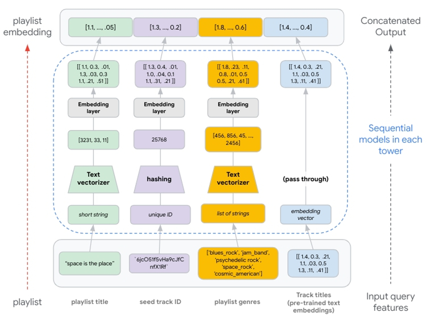 |
| Figure 8: Illustration of feature processing from input to concatenated output. Text features are generated via n-grams. Integer indexes of n-grams are passed to an embedding layer. Hashing produces unique integers up to 1,000,000; values passed to an embedding layer. If using pre-trained embeddings, these are passed through the tower without transformation and concatenated with the other embedding representations. |
Hashing vs StringLookup() layers
Hashing is generally recommended when fast performance is needed and is preferred over string lookups because it skips the need for a lookup table. Setting the proper bin size for the hashing layer is critical. When there are more unique values than hashing bins, values start getting placed into the same bins, and this can negatively impact our recommendations. This is commonly referred to as a hashing collision, and can be avoided when building the model by allocating enough bins for the unique values. See turning categorical features into embeddings for more details.
TextVectorization() layers
The key to text features is to understand if creating additional NLP features with the TextVectorization layer is helpful. If additional context derived from the text feature is minimal, it may not be worth the cost to model training. This layer needs to be adapted from the source dataset, meaning the layer requires a scan of the training data to create lookup dictionaries for the top N n-grams (set by max_tokens).
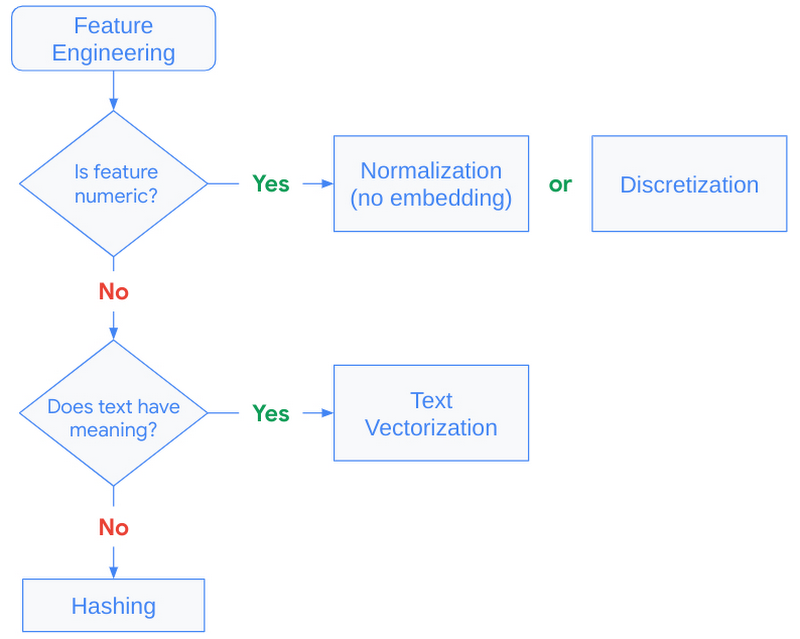 |
| Figure 9: Decision tree to guide feature engineering strategy. |
Efficient retrieval with Matching Engine
So far we’ve discussed how to map queries and candidates to the shared embedding space. Now let’s discuss how to best use this shared embedding space for efficient serving.
Recall at serving time, we will use the trained query tower to compute the embeddings for a query (playlist) and use this embedding vector in a nearest neighbor search for the most similar candidate (track) embeddings. And, because the candidate dataset can grow to millions or billions of vectors, this nearest neighbor search often becomes a computational bottleneck for low-latency inference.
Many state-of-the-art techniques address the computational bottleneck by compressing the candidate vectors such that ANN calculations can be performed in a fraction of the time needed for an exhaustive search. The novel compression algorithm proposed by Google Research modifies these techniques to also optimize for the nearest neighbor search accuracy. The details of their proposed technique are described here, but fundamentally their approach seeks to compress the candidate vectors such that the original distances between vectors are preserved. Compared to previous solutions, this results in a more accurate relative ranking of a vector and its nearest neighbors, i.e., it minimizes distorting the vector similarities our model learned from the training data.
Fully managed vector database and ANN service
Matching Engine is a managed solution utilizing these techniques for efficient vector similarity search. It offers customers a highly scalable vector database and ANN service while alleviating the operational overhead of developing and maintaining similar solutions, such as the open sourced ScaNN library. It includes several capabilities that simplify production deployments, including:
- Large-scale: supports large embedding datasets with up to 1 billion embedding vectors
- Incremental updates: depending on the number of vectors, complete index rebuilds can take hours. With incremental updates, customers can make small changes without building a new index (see Update and rebuild an active index for more details)
- Dynamic rebuilds: when an index grows beyond its original configuration, Matching Engine periodically re-organizes the index and serving structure to ensure optimal performance
- Autoscaling: underlying infrastructure is autoscaled to ensure consistent performance at scale
- Filtering and diversity: ability to include multiple restrict and crowding tags per vector. At query inference time, use boolean predicates to filter and diversify retrieved candidates (see Filter vector matches for more details)
When creating an ANN index, Matching Engine uses the Tree-AH strategy to build a distributed implementation of our candidate index. It combines two algorithms:
- Distributed search tree for hierarchically organizing the embedding space. Each level of this tree is a clustering of the nodes at the next level down, where the final leaf-level is a clustering of our candidate embedding vectors
- Asymmetric hashing (AH) for fast dot product approximation algorithm used to score similarity between a query vector and the search tree nodes
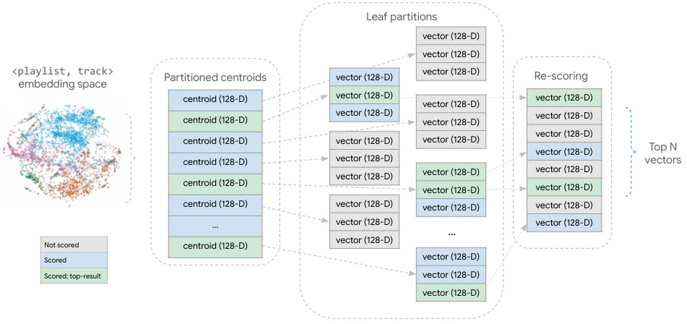 |
| Figure 10: conceptual representation of the partitioned candidate vector dataset. During query inference, all partition centroids are scored. In the centroids most similar to the query vector, all candidate vectors are scored. The scored candidate vectors are aggregated and re-scored, returning the top N candidate vectors. |
This strategy shards our embedding vectors into partitions, where each partition is represented by the centroid of the vectors it contains. The aggregate of these partition centroids form a smaller dataset summarizing the larger, distributed vector dataset. At inference time, Matching Engine scores all the partitioned centroids, then scores the vectors within the partitions whose centroids are most similar to the query vector.
Conclusion
In this blog we took a deep dive into understanding critical components of a candidate retrieval workflow using TensorFlow Recommenders and Vertex AI Matching Engine. We took a closer look at the foundational concepts of two-tower architectures, explored the semantics of query and candidate entities, and discussed how things like the structure of training examples can impact the success of candidate retrieval.
In a subsequent post we will demonstrate how to use Vertex AI and other Google Cloud services to implement these techniques at scale. We’ll show how to leverage BigQuery and Dataflow to structure training examples and convert them to TFRecords for model training. We’ll outline how to structure a Python application for training two-tower models with the Vertex AI Training service. And we’ll detail the steps for operationalizing the trained towers.
Now Shipping: DGX H100 Systems Bring Advanced AI Capabilities to Industries Worldwide
Customers from Japan to Ecuador and Sweden are using NVIDIA DGX H100 systems like AI factories to manufacture intelligence.
They’re creating services that offer AI-driven insights in finance, healthcare, law, IT and telecom — and working to transform their industries in the process.
Among the dozens of use cases, one aims to predict how factory equipment will age, so tomorrow’s plants can be more efficient.
Called Green Physics AI, it adds information like an object’s CO2 footprint, age and energy consumption to SORDI.ai, which claims to be the largest synthetic dataset in manufacturing.
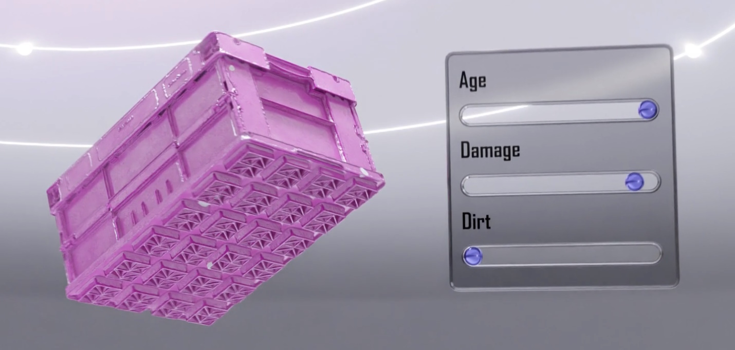
The dataset lets manufacturers develop powerful AI models and create digital twins that optimize the efficiency of factories and warehouses. With Green Physics AI, they also can optimize energy and CO2 savings for the factory’s products and the components that go into them.
Meet Your Smart Valet
Imagine a robot that could watch you wash dishes or change the oil in your car, then do it for you.
Boston Dynamics AI Institute (The AI Institute), a research organization which traces its roots to Boston Dynamics, the well-known pioneer in robotics, will use a DGX H100 to pursue that vision. Researchers imagine dexterous mobile robots helping people in factories, warehouses, disaster sites and eventually homes.
“One thing I’ve dreamed about since I was in grad school is a robot valet who can follow me and do useful tasks — everyone should have one,” said Al Rizzi, CTO of The AI Institute.
That will require breakthroughs in AI and robotics, something Rizzi has seen firsthand. As chief scientist at Boston Dynamics, he helped create robots like Spot, a quadruped that can navigate stairs and even open doors for itself.
Initially, the DGX H100 will tackle tasks in reinforcement learning, a key technique in robotics. Later, it will run AI inference jobs while connected directly to prototype bots in the lab.
“It’s an extremely high-performance computer in a relatively compact footprint, so it provides an easy way for us to develop and deploy AI models,” said Rizzi.
Born to Run Gen AI
You don’t have to be a world-class research outfit or Fortune 500 company to use a DGX H100. Startups are unboxing some of the first systems to ride the wave of generative AI.
For example, Scissero, with offices in London and New York, employs a GPT-powered chatbot to make legal processes more efficient. Its Scissero GPT can draft legal documents, generate reports and conduct legal research.
In Germany, DeepL will use several DGX H100 systems to expand services like translation between dozens of languages it provides for customers, including Nikkei, Japan’s largest publishing company. DeepL recently released an AI writing assistant called DeepL Write.
Here’s to Your Health
Many of the DGX H100 systems will advance healthcare and improve patient outcomes.
In Tokyo, DGX H100s will run simulations and AI to speed the drug discovery process as part of the Tokyo-1 supercomputer. Xeureka — a startup launched in November 2021 by Mitsui & Co. Ltd., one of Japan’s largest conglomerates — will manage the system.
Separately, hospitals and academic healthcare organizations in Germany, Israel and the U.S. will be among the first users of DGX H100 systems.
Lighting Up Around the Globe
Universities from Singapore to Sweden are plugging in DGX H100 systems for research across a range of fields.
A DGX H100 will train large language models for Johns Hopkins University Applied Physics Laboratory. The KTH Royal Institute of Sweden will use one to expand its supercomputing capabilities.
Among other use cases, Japan’s CyberAgent, an internet services company, is creating smart digital ads and celebrity avatars. Telconet, a leading telecommunications provider in Ecuador, is building intelligent video analytics for safe cities and language services to support customers across Spanish dialects.
An Engine of AI Innovation
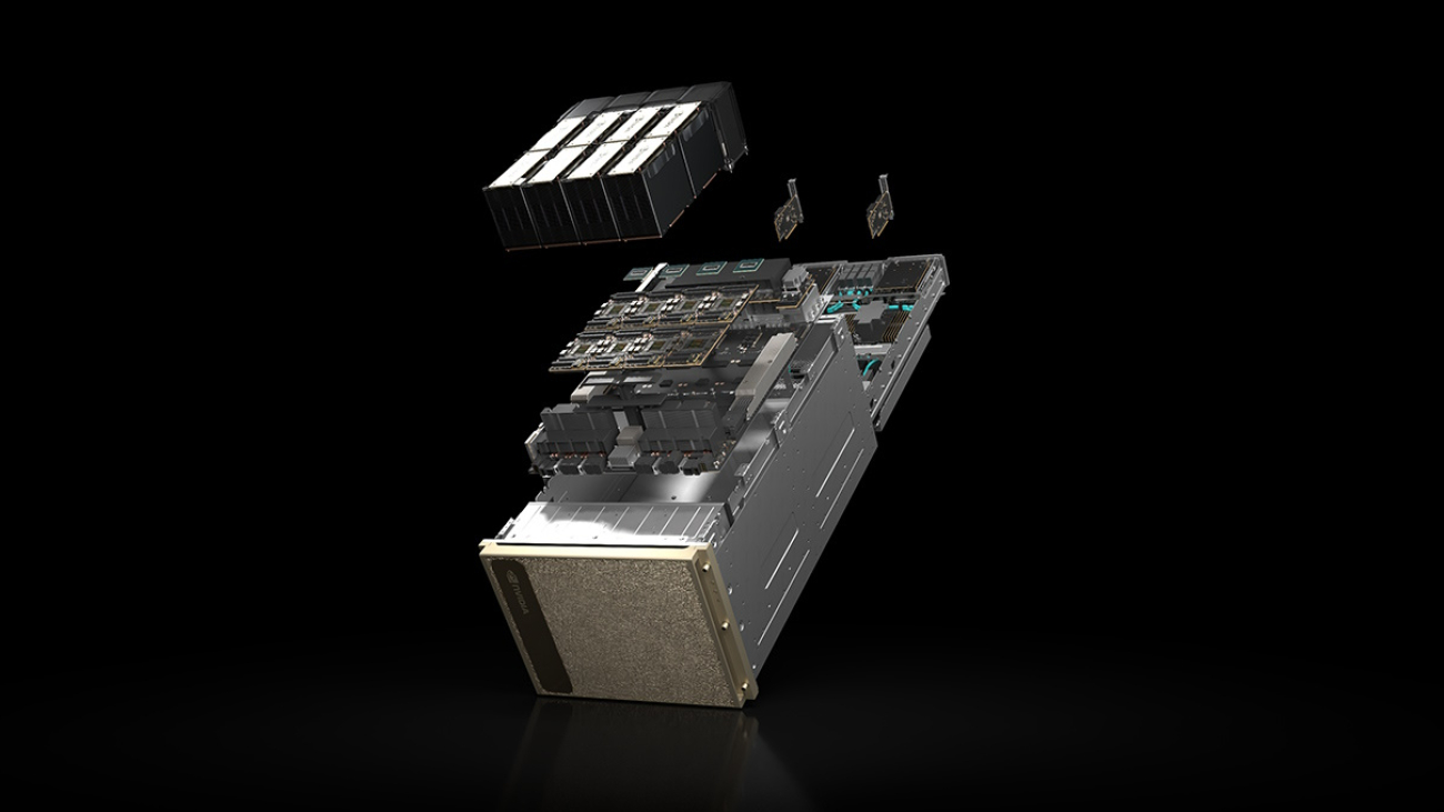
Each NVIDIA H100 Tensor Core GPU in a DGX H100 system provides on average about 6x more performance than prior GPUs. A DGX H100 packs eight of them, each with a Transformer Engine designed to accelerate generative AI models.
The eight H100 GPUs connect over NVIDIA NVLink to create one giant GPU. Scaling doesn’t stop there: organizations can connect hundreds of DGX H100 nodes into an AI supercomputer using the 400 Gbps ultra-low latency NVIDIA Quantum InfiniBand, twice the speed of prior networks.
Fueled by a Full Software Stack
DGX H100 systems run on NVIDIA Base Command, a suite for accelerating compute, storage, and network infrastructure and optimizing AI workloads.
They also include NVIDIA AI Enterprise, software to accelerate data science pipelines and streamline development and deployment of generative AI, computer vision and more.
The DGX platform offers both high performance and efficiency. DGX H100 delivers a 2x improvement in kilowatts per petaflop over the DGX A100 generation.
NVIDIA DGX H100 systems, DGX PODs and DGX SuperPODs are available from NVIDIA’s global partners.
Manuvir Das, NVIDIA’s vice president of enterprise computing, announced DGX H100 systems are shipping in a talk at MIT Technology Review’s Future Compute event today. A link to his talk will be available here soon.

Google at ICLR 2023

The Eleventh International Conference on Learning Representations (ICLR 2023) is being held this week as a hybrid event in Kigali, Rwanda. We are proud to be a Diamond Sponsor of ICLR 2023, a premier conference on deep learning, where Google researchers contribute at all levels. This year we are presenting over 100 papers and are actively involved in organizing and hosting a number of different events, including workshops and interactive sessions.
If you’re registered for ICLR 2023, we hope you’ll visit the Google booth to learn more about the exciting work we’re doing across topics spanning representation and reinforcement learning, theory and optimization, social impact, safety and privacy, and applications from generative AI to speech and robotics. Continue below to find the many ways in which Google researchers are engaged at ICLR 2023, including workshops, papers, posters and talks (Google affiliations in bold).
Board and Organizing Committee
Board Members include: Shakir Mohamed, Tara Sainath
Senior Program Chairs include: Been Kim
Workshop Chairs include: Aisha Walcott-Bryant, Rose Yu
Diversity, Equity & Inclusion Chairs include: Rosanne Liu
Outstanding Paper awards
Emergence of Maps in the Memories of Blind Navigation Agents
Erik Wijmans, Manolis Savva, Irfan Essa, Stefan Lee, Ari S. Morcos, Dhruv Batra
DreamFusion: Text-to-3D Using 2D Diffusion
Ben Poole, Ajay Jain, Jonathan T. Barron, Ben Mildenhall
Keynote speaker
Learned Optimizers: Why They’re the Future, Why They’re Hard, and What They Can Do Now
Jascha Sohl-Dickstein
Workshops
Kaggle@ICLR 2023: ML Solutions in Africa
Organizers include: Julia Elliott, Phil Culliton, Ray Harvey
Facilitators: Julia Elliot, Walter Reade
Reincarnating Reinforcement Learning (Reincarnating RL)
Organizers include: Rishabh Agarwal, Ted Xiao, Max Schwarzer
Speakers include: Sergey Levine
Panelists include: Marc G. Bellemare, Sergey Levine
Trustworthy and Reliable Large-Scale Machine Learning Models
Organizers include: Sanmi Koyejo
Speakers include: Nicholas Carlini
Physics for Machine Learning (Physics4ML)
Speakers include: Yasaman Bahri
AI for Agent-Based Modelling Community (AI4ABM)
Organizers include: Pablo Samuel Castro
Mathematical and Empirical Understanding of Foundation Models (ME-FoMo)
Organizers include: Mathilde Caron, Tengyu Ma, Hanie Sedghi
Speakers include: Yasaman Bahri, Yann Dauphin
Neurosymbolic Generative Models 2023 (NeSy-GeMs)
Organizers include: Kevin Ellis
Speakers include: Daniel Tarlow, Tuan Anh Le
What Do We Need for Successful Domain Generalization?
Panelists include: Boqing Gong
The 4th Workshop on Practical ML for Developing Countries: Learning Under Limited/Low Resource Settings
Keynote Speaker: Adji Bousso Dieng
Machine Learning for Remote Sensing
Speakers include: Abigail Annkah
Multimodal Representation Learning (MRL): Perks and Pitfalls
Organizers include: Petra Poklukar
Speakers include: Arsha Nagrani
Pitfalls of Limited Data and Computation for Trustworthy ML
Organizers include: Prateek Jain
Speakers include: Nicholas Carlini, Praneeth Netrapalli
Sparsity in Neural Networks: On Practical Limitations and Tradeoffs Between Sustainability and Efficiency
Organizers include: Trevor Gale, Utku Evci
Speakers include: Aakanksha Chowdhery, Jeff Dean
Time Series Representation Learning for Health
Speakers include: Katherine Heller
Deep Learning for Code (DL4C)
Organizers include: Gabriel Orlanski
Speakers include: Alex Polozov, Daniel Tarlow
Affinity Workshops
Tiny Papers Showcase Day (a DEI initiative)
Organizers include: Rosanne Liu
Papers
Evolve Smoothly, Fit Consistently: Learning Smooth Latent Dynamics for Advection-Dominated Systems
Zhong Yi Wan, Leonardo Zepeda-Nunez, Anudhyan Boral, Fei Sha
Quantifying Memorization Across Neural Language Models
Nicholas Carlini, Daphne Ippolito, Matthew Jagielski, Katherine Lee, Florian Tramer, Chiyuan Zhang
Emergence of Maps in the Memories of Blind Navigation Agents (Outstanding Paper Award)
Erik Wijmans, Manolis Savva, Irfan Essa, Stefan Lee, Ari S. Morcos, Dhruv Batra
Offline Q-Learning on Diverse Multi-task Data Both Scales and Generalizes (see blog post)
Aviral Kumar, Rishabh Agarwal, Xingyang Geng, George Tucker, Sergey Levine
ReAct: Synergizing Reasoning and Acting in Language Models (see blog post)
Shunyu Yao*, Jeffrey Zhao, Dian Yu, Nan Du, Izhak Shafran, Karthik R. Narasimhan, Yuan Cao
Prompt-to-Prompt Image Editing with Cross-Attention Control
Amir Hertz, Ron Mokady, Jay Tenenbaum, Kfir Aberman, Yael Pritch, Daniel Cohen-Or
DreamFusion: Text-to-3D Using 2D Diffusion (Outstanding Paper Award)
Ben Poole, Ajay Jain, Jonathan T. Barron, Ben Mildenhall
A System for Morphology-Task Generalization via Unified Representation and Behavior Distillation
Hiroki Furuta, Yusuke Iwasawa, Yutaka Matsuo, Shixiang Shane Gu
Sample-Efficient Reinforcement Learning by Breaking the Replay Ratio Barrier
Pierluca D’Oro, Max Schwarzer, Evgenii Nikishin, Pierre-Luc Bacon, Marc G Bellemare, Aaron Courville
Dichotomy of Control: Separating What You Can Control from What You Cannot
Sherry Yang, Dale Schuurmans, Pieter Abbeel, Ofir Nachum
Fast and Precise: Adjusting Planning Horizon with Adaptive Subgoal Search
Michał Zawalski, Michał Tyrolski, Konrad Czechowski, Tomasz Odrzygóźdź, Damian Stachura, Piotr Piekos, Yuhuai Wu, Łukasz Kucinski, Piotr Miłos
The Trade-Off Between Universality and Label Efficiency of Representations from Contrastive Learning
Zhenmei Shi, Jiefeng Chen, Kunyang Li, Jayaram Raghuram, Xi Wu, Yingyu Liang, Somesh Jha
Sparsity-Constrained Optimal Transport
Tianlin Liu*, Joan Puigcerver, Mathieu Blondel
Unmasking the Lottery Ticket Hypothesis: What’s Encoded in a Winning Ticket’s Mask?
Mansheej Paul, Feng Chen, Brett W. Larsen, Jonathan Frankle, Surya Ganguli, Gintare Karolina Dziugaite
Extreme Q-Learning: MaxEnt RL without Entropy
Divyansh Garg, Joey Hejna, Matthieu Geist, Stefano Ermon
Draft, Sketch, and Prove: Guiding Formal Theorem Provers with Informal Proofs
Albert Qiaochu Jiang, Sean Welleck, Jin Peng Zhou, Timothee Lacroix, Jiacheng Liu, Wenda Li, Mateja Jamnik, Guillaume Lample, Yuhuai Wu
SimPer: Simple Self-Supervised Learning of Periodic Targets
Yuzhe Yang, Xin Liu, Jiang Wu, Silviu Borac, Dina Katabi, Ming-Zher Poh, Daniel McDuff
Socratic Models: Composing Zero-Shot Multimodal Reasoning with Language
Andy Zeng, Maria Attarian, Brian Ichter, Krzysztof Marcin Choromanski, Adrian Wong, Stefan Welker, Federico Tombari, Aveek Purohit, Michael S. Ryoo, Vikas Sindhwani, Johnny Lee, Vincent Vanhoucke, Pete Florence
What Learning Algorithm Is In-Context Learning? Investigations with Linear Models
Ekin Akyurek*, Dale Schuurmans, Jacob Andreas, Tengyu Ma*, Denny Zhou
Preference Transformer: Modeling Human Preferences Using Transformers for RL
Changyeon Kim, Jongjin Park, Jinwoo Shin, Honglak Lee, Pieter Abbeel, Kimin Lee
Iterative Patch Selection for High-Resolution Image Recognition
Benjamin Bergner, Christoph Lippert, Aravindh Mahendran
Open-Vocabulary Object Detection upon Frozen Vision and Language Models
Weicheng Kuo, Yin Cui, Xiuye Gu, AJ Piergiovanni, Anelia Angelova
(Certified!!) Adversarial Robustness for Free!
Nicholas Carlini, Florian Tramér, Krishnamurthy (Dj) Dvijotham, Leslie Rice, Mingjie Sun, J. Zico Kolter
REPAIR: REnormalizing Permuted Activations for Interpolation Repair
Keller Jordan, Hanie Sedghi, Olga Saukh, Rahim Entezari, Behnam Neyshabur
Discrete Predictor-Corrector Diffusion Models for Image Synthesis
José Lezama, Tim Salimans, Lu Jiang, Huiwen Chang, Jonathan Ho, Irfan Essa
Feature Reconstruction From Outputs Can Mitigate Simplicity Bias in Neural Networks
Sravanti Addepalli, Anshul Nasery, Praneeth Netrapalli, Venkatesh Babu R., Prateek Jain
An Exact Poly-time Membership-Queries Algorithm for Extracting a Three-Layer ReLU Network
Amit Daniely, Elad Granot
Language Models Are Multilingual Chain-of-Thought Reasoners
Freda Shi, Mirac Suzgun, Markus Freitag, Xuezhi Wang, Suraj Srivats, Soroush Vosoughi, Hyung Won Chung, Yi Tay, Sebastian Ruder, Denny Zhou, Dipanjan Das, Jason Wei
Scaling Forward Gradient with Local Losses
Mengye Ren*, Simon Kornblith, Renjie Liao, Geoffrey Hinton
Treeformer: Dense Gradient Trees for Efficient Attention Computation
Lovish Madaan, Srinadh Bhojanapalli, Himanshu Jain, Prateek Jain
LilNetX: Lightweight Networks with EXtreme Model Compression and Structured Sparsification
Sharath Girish, Kamal Gupta, Saurabh Singh, Abhinav Shrivastava
DiffusER: Diffusion via Edit-Based Reconstruction
Machel Reid, Vincent J. Hellendoorn, Graham Neubig
Leveraging Unlabeled Data to Track Memorization
Mahsa Forouzesh, Hanie Sedghi, Patrick Thiran
A Mixture-of-Expert Approach to RL-Based Dialogue Management
Yinlam Chow, Aza Tulepbergenov, Ofir Nachum, Dhawal Gupta, Moonkyung Ryu, Mohammad Ghavamzadeh, Craig Boutilier
Easy Differentially Private Linear Regression
Kareem Amin, Matthew Joseph, Monica Ribero, Sergei Vassilvitskii
KwikBucks: Correlation Clustering with Cheap-Weak and Expensive-Strong Signals
Sandeep Silwal*, Sara Ahmadian, Andrew Nystrom, Andrew McCallum, Deepak Ramachandran, Mehran Kazemi
Massively Scaling Heteroscedastic Classifiers
Mark Collier, Rodolphe Jenatton, Basil Mustafa, Neil Houlsby, Jesse Berent, Effrosyni Kokiopoulou
The Lazy Neuron Phenomenon: On Emergence of Activation Sparsity in Transformers
Zonglin Li, Chong You, Srinadh Bhojanapalli, Daliang Li, Ankit Singh Rawat, Sashank J. Reddi, Ke Ye, Felix Chern, Felix Yu, Ruiqi Guo, Sanjiv Kumar
Compositional Semantic Parsing with Large Language Models
Andrew Drozdov, Nathanael Scharli, Ekin Akyurek, Nathan Scales, Xinying Song, Xinyun Chen, Olivier Bousquet, Denny Zhou
Extremely Simple Activation Shaping for Out-of-Distribution Detection
Andrija Djurisic, Nebojsa Bozanic, Arjun Ashok, Rosanne Liu
Long Range Language Modeling via Gated State Spaces
Harsh Mehta, Ankit Gupta, Ashok Cutkosky, Behnam Neyshabur
Investigating Multi-task Pretraining and Generalization in Reinforcement Learning
Adrien Ali Taiga, Rishabh Agarwal, Jesse Farebrother, Aaron Courville, Marc G. Bellemare
Learning Low Dimensional State Spaces with Overparameterized Recurrent Neural Nets
Edo Cohen-Karlik, Itamar Menuhin-Gruman, Raja Giryes, Nadav Cohen, Amir Globerson
Weighted Ensemble Self-Supervised Learning
Yangjun Ruan*, Saurabh Singh, Warren Morningstar, Alexander A. Alemi, Sergey Ioffe, Ian Fischer, Joshua V. Dillon
Calibrating Sequence Likelihood Improves Conditional Language Generation
Yao Zhao, Misha Khalman, Rishabh Joshi, Shashi Narayan, Mohammad Saleh, Peter J. Liu
SMART: Sentences as Basic Units for Text Evaluation
Reinald Kim Amplayo, Peter J. Liu, Yao Zhao, Shashi Narayan
Leveraging Importance Weights in Subset Selection
Gui Citovsky, Giulia DeSalvo, Sanjiv Kumar, Srikumar Ramalingam, Afshin Rostamizadeh, Yunjuan Wang*
Proto-Value Networks: Scaling Representation Learning with Auxiliary Tasks
Jesse Farebrother, Joshua Greaves, Rishabh Agarwal, Charline Le Lan, Ross Goroshin, Pablo Samuel Castro, Marc G. Bellemare
An Extensible Multi-modal Multi-task Object Dataset with Materials
Trevor Standley, Ruohan Gao, Dawn Chen, Jiajun Wu, Silvio Savarese
Measuring Forgetting of Memorized Training Examples
Matthew Jagielski, Om Thakkar, Florian Tramér, Daphne Ippolito, Katherine Lee, Nicholas Carlini, Eric Wallace, Shuang Song, Abhradeep Thakurta, Nicolas Papernot, Chiyuan Zhang
Bidirectional Language Models Are Also Few-Shot Learners
Ajay Patel, Bryan Li, Mohammad Sadegh Rasooli, Noah Constant, Colin Raffel, Chris Callison-Burch
Is Attention All That NeRF Needs?
Mukund Varma T., Peihao Wang, Xuxi Chen, Tianlong Chen, Subhashini Venugopalan, Zhangyang Wang
Automating Nearest Neighbor Search Configuration with Constrained Optimization
Philip Sun, Ruiqi Guo, Sanjiv Kumar
Static Prediction of Runtime Errors by Learning to Execute Programs with External Resource Descriptions
David Bieber, Rishab Goel, Daniel Zheng, Hugo Larochelle, Daniel Tarlow
Composing Ensembles of Pre-trained Models via Iterative Consensus
Shuang Li, Yilun Du, Joshua B. Tenenbaum, Antonio Torralba, Igor Mordatch
Λ-DARTS: Mitigating Performance Collapse by Harmonizing Operation Selection Among Cells
Sajad Movahedi, Melika Adabinejad, Ayyoob Imani, Arezou Keshavarz, Mostafa Dehghani, Azadeh Shakery, Babak N. Araabi
Blurring Diffusion Models
Emiel Hoogeboom, Tim Salimans
Part-Based Models Improve Adversarial Robustness
Chawin Sitawarin, Kornrapat Pongmala, Yizheng Chen, Nicholas Carlini, David Wagner
Learning in Temporally Structured Environments
Matt Jones, Tyler R. Scott, Mengye Ren, Gamaleldin ElSayed, Katherine Hermann, David Mayo, Michael C. Mozer
SlotFormer: Unsupervised Visual Dynamics Simulation with Object-Centric Models
Ziyi Wu, Nikita Dvornik, Klaus Greff, Thomas Kipf, Animesh Garg
Robust Algorithms on Adaptive Inputs from Bounded Adversaries
Yeshwanth Cherapanamjeri, Sandeep Silwal, David P. Woodruff, Fred Zhang, Qiuyi (Richard) Zhang, Samson Zhou
Agnostic Learning of General ReLU Activation Using Gradient Descent
Pranjal Awasthi, Alex Tang, Aravindan Vijayaraghavan
Analog Bits: Generating Discrete Data Using Diffusion Models with Self-Conditioning
Ting Chen, Ruixiang Zhang, Geoffrey Hinton
Any-Scale Balanced Samplers for Discrete Space
Haoran Sun*, Bo Dai, Charles Sutton, Dale Schuurmans, Hanjun Dai
Augmentation with Projection: Towards an Effective and Efficient Data Augmentation Paradigm for Distillation
Ziqi Wang*, Yuexin Wu, Frederick Liu, Daogao Liu, Le Hou, Hongkun Yu, Jing Li, Heng Ji
Beyond Lipschitz: Sharp Generalization and Excess Risk Bounds for Full-Batch GD
Konstantinos E. Nikolakakis, Farzin Haddadpour, Amin Karbasi, Dionysios S. Kalogerias
Causal Estimation for Text Data with (Apparent) Overlap Violations
Lin Gui, Victor Veitch
Contrastive Learning Can Find an Optimal Basis for Approximately View-Invariant Functions
Daniel D. Johnson, Ayoub El Hanchi, Chris J. Maddison
Differentially Private Adaptive Optimization with Delayed Preconditioners
Tian Li, Manzil Zaheer, Ziyu Liu, Sashank Reddi, Brendan McMahan, Virginia Smith
Distributionally Robust Post-hoc Classifiers Under Prior Shifts
Jiaheng Wei*, Harikrishna Narasimhan, Ehsan Amid, Wen-Sheng Chu, Yang Liu, Abhishek Kumar
Human Alignment of Neural Network Representations
Lukas Muttenthaler, Jonas Dippel, Lorenz Linhardt, Robert A. Vandermeulen, Simon Kornblith
Implicit Bias in Leaky ReLU Networks Trained on High-Dimensional Data
Spencer Frei, Gal Vardi, Peter Bartlett, Nathan Srebro, Wei Hu
Koopman Neural Operator Forecaster for Time-Series with Temporal Distributional Shifts
Rui Wang*, Yihe Dong, Sercan Ö. Arik, Rose Yu
Latent Variable Representation for Reinforcement Learning
Tongzheng Ren, Chenjun Xiao, Tianjun Zhang, Na Li, Zhaoran Wang, Sujay Sanghavi, Dale Schuurmans, Bo Dai
Least-to-Most Prompting Enables Complex Reasoning in Large Language Models
Denny Zhou, Nathanael Scharli, Le Hou, Jason Wei, Nathan Scales, Xuezhi Wang, Dale Schuurmans, Claire Cui, Olivier Bousquet, Quoc Le, Ed Chi
Mind’s Eye: Grounded Language Model Reasoning Through Simulation
Ruibo Liu, Jason Wei, Shixiang Shane Gu, Te-Yen Wu, Soroush Vosoughi, Claire Cui, Denny Zhou, Andrew M. Dai
MOAT: Alternating Mobile Convolution and Attention Brings Strong Vision Models
Chenglin Yang*, Siyuan Qiao, Qihang Yu, Xiaoding Yuan, Yukun Zhu, Alan Yuille, Hartwig Adam, Liang-Chieh Chen
Novel View Synthesis with Diffusion Models
Daniel Watson, William Chan, Ricardo Martin-Brualla, Jonathan Ho, Andrea Tagliasacchi, Mohammad Norouzi
On Accelerated Perceptrons and Beyond
Guanghui Wang, Rafael Hanashiro, Etash Guha, Jacob Abernethy
On Compositional Uncertainty Quantification for Seq2seq Graph Parsing
Zi Lin*, Du Phan, Panupong Pasupat, Jeremiah Liu, Jingbo Shang
On the Robustness of Safe Reinforcement Learning Under Observational Perturbations
Zuxin Liu, Zijian Guo, Zhepeng Cen, Huan Zhang, Jie Tan, Bo Li, Ding Zhao
Online Low Rank Matrix Completion
Prateek Jain, Soumyabrata Pal
Out-of-Distribution Detection and Selective Generation for Conditional Language Models
Jie Ren, Jiaming Luo, Yao Zhao, Kundan Krishna*, Mohammad Saleh, Balaji Lakshminarayanan, Peter J. Liu
PaLI: A Jointly-Scaled Multilingual Language-Image Model
Xi Chen, Xiao Wang, Soravit Changpinyo, AJ Piergiovanni, Piotr Padlewski, Daniel Salz, Sebastian Goodman, Adam Grycner, Basil Mustafa, Lucas Beyer, Alexander Kolesnikov, Joan Puigcerver, Nan Ding, Keran Rong, Hassan Akbari, Gaurav Mishra, Linting Xue, Ashish V. Thapliyal, James Bradbury, Weicheng Kuo, Mojtaba Seyedhosseini, Chao Jia, Burcu Karagol Ayan, Carlos Riquelme Ruiz, Andreas Peter Steiner, Anelia Angelova, Xiaohua Zhai, Neil Houlsby, Radu Soricut
Phenaki: Variable Length Video Generation from Open Domain Textual Descriptions
Ruben Villegas, Mohammad Babaeizadeh, Pieter-Jan Kindermans, Hernan Moraldo, Han Zhang, Mohammad Taghi Saffar, Santiago Castro*, Julius Kunze*, Dumitru Erhan
Promptagator: Few-Shot Dense Retrieval from 8 Examples
Zhuyun Dai, Vincent Y. Zhao, Ji Ma, Yi Luan, Jianmo Ni, Jing Lu, Anton Bakalov, Kelvin Guu, Keith B. Hall, Ming-Wei Chang
Pushing the Accuracy-Group Robustness Frontier with Introspective Self-Play
Jeremiah Zhe Liu, Krishnamurthy Dj Dvijotham, Jihyeon Lee, Quan Yuan, Balaji Lakshminarayanan, Deepak Ramachandran
Re-Imagen: Retrieval-Augmented Text-to-Image Generator
Wenhu Chen, Hexiang Hu, Chitwan Saharia, William W. Cohen
Recitation-Augmented Language Models
Zhiqing Sun, Xuezhi Wang, Yi Tay, Yiming Yang, Denny Zhou
Regression with Label Differential Privacy
Badih Ghazi, Pritish Kamath, Ravi Kumar, Ethan Leeman, Pasin Manurangsi, Avinash Varadarajan, Chiyuan Zhang
Revisiting the Entropy Semiring for Neural Speech Recognition
Oscar Chang, Dongseong Hwang, Olivier Siohan
Robust Active Distillation
Cenk Baykal, Khoa Trinh, Fotis Iliopoulos, Gaurav Menghani, Erik Vee
Score-Based Continuous-Time Discrete Diffusion Models
Haoran Sun*, Lijun Yu, Bo Dai, Dale Schuurmans, Hanjun Dai
Self-Consistency Improves Chain of Thought Reasoning in Language Models
Xuezhi Wang, Jason Wei, Dale Schuurmans, Quoc Le, Ed H. Chi, Sharan Narang, Aakanksha Chowdhery, Denny Zhou
Self-Supervision Through Random Segments with Autoregressive Coding (RandSAC)
Tianyu Hua, Yonglong Tian, Sucheng Ren, Michalis Raptis, Hang Zhao, Leonid Sigal
Serving Graph Compression for Graph Neural Networks
Si Si, Felix Yu, Ankit Singh Rawat, Cho-Jui Hsieh, Sanjiv Kumar
Sequential Attention for Feature Selection
Taisuke Yasuda*, MohammadHossein Bateni, Lin Chen, Matthew Fahrbach, Gang Fu, Vahab Mirrokni
Sparse Upcycling: Training Mixture-of-Experts from Dense Checkpoints
Aran Komatsuzaki*, Joan Puigcerver, James Lee-Thorp, Carlos Riquelme, Basil Mustafa, Joshua Ainslie, Yi Tay, Mostafa Dehghani, Neil Houlsby
Spectral Decomposition Representation for Reinforcement Learning
Tongzheng Ren, Tianjun Zhang, Lisa Lee, Joseph Gonzalez, Dale Schuurmans, Bo Dai
Spotlight: Mobile UI Understanding Using Vision-Language Models with a Focus (see blog post)
Gang Li, Yang Li
Supervision Complexity and Its Role in Knowledge Distillation
Hrayr Harutyunyan*, Ankit Singh Rawat, Aditya Krishna Menon, Seungyeon Kim, Sanjiv Kumar
Teacher Guided Training: An Efficient Framework for Knowledge Transfer
Manzil Zaheer, Ankit Singh Rawat, Seungyeon Kim, Chong You, Himanshu Jain, Andreas Veit, Rob Fergus, Sanjiv Kumar
TEMPERA: Test-Time Prompt Editing via Reinforcement Learning
Tianjun Zhang, Xuezhi Wang, Denny Zhou, Dale Schuurmans, Joseph E. Gonzalez
UL2: Unifying Language Learning Paradigms
Yi Tay, Mostafa Dehghani, Vinh Q. Tran, Xavier Garcia, Jason Wei, Xuezhi Wang, Hyung Won Chung, Dara Bahri, Tal Schuster, Steven Zheng, Denny Zhou, Neil Houlsby, Donald Metzler
* Work done while at Google