Monthly Archives: June 2023

You can now retrain machine learning (ML) models and automate batch prediction workflows with updated datasets in Amazon SageMaker Canvas, thereby making it easier to constantly learn and improve the model performance and drive efficiency. An ML model’s effectiveness depends on the quality and relevance of the data it’s trained on. As time progresses, the underlying patterns, trends, and distributions in the data may change. By updating the dataset, you ensure that the model learns from the most recent and representative data, thereby improving its ability to make accurate predictions. Canvas now supports updating datasets automatically and manually enabling you to use the latest version of the tabular, image, and document dataset for training ML models.

After the model is trained, you may want to run predictions on it. Running batch predictions on an ML model enables processing multiple data points simultaneously instead of making predictions one by one. Automating this process provides efficiency, scalability, and timely decision-making. After the predictions are generated, they can be further analyzed, aggregated, or visualized to gain insights, identify patterns, or make informed decisions based on the predicted outcomes. Canvas now supports setting up an automated batch prediction configuration and associating a dataset to it. When the associated dataset is refreshed, either manually or on a schedule, a batch prediction workflow will be triggered automatically on the corresponding model. Results of the predictions can be viewed inline or downloaded for later review.

In this post, we show how to retrain ML models and automate batch predictions using updated datasets in Canvas.

Overview of solution

For our use case, we play the part of a business analyst for an ecommerce company. Our product team wants us to determine the most critical metrics that influence a shopper’s purchase decision. For this, we train an ML model in Canvas with a customer website online session dataset from the company. We evaluate the model’s performance and, if needed, retrain the model with additional data to see if it improves the performance of the existing model or not. To do so, we use the auto update dataset capability in Canvas and retrain our existing ML model with the latest version of training dataset. Then we configure automatic batch prediction workflows—when the corresponding prediction dataset is updated, it automatically triggers the batch prediction job on the model and makes the results available for us to review.

The workflow steps are as follows:

1. Upload the downloaded customer website online session data to Amazon Simple Storage Service (Amazon S3) and create a new training dataset Canvas. For the full list of supported data sources, refer to Importing data in Amazon SageMaker Canvas.
2. Build ML models and analyze their performance metrics. Refer to the steps on how to build a custom ML Model in Canvas and evaluate a model’s performance.
3. Set up auto update on the existing training dataset and upload new data to the Amazon S3 location backing this dataset. Upon completion, it should create a new dataset version.
4. Use the latest version of the dataset to retrain the ML model and analyze its performance.
5. Set up automatic batch predictions on the better performing model version and view the prediction results.

You can perform these steps in Canvas without writing a single line of code.

Overview of data

The dataset consists of feature vectors belonging to 12,330 sessions. The dataset was formed so that each session would belong to a different user in a 1-year period to avoid any tendency to a specific campaign, special day, user profile, or period. The following table outlines the data schema.

Revenue is the target column, which will help us predict whether or not a shopper will purchase a product or not.

The first step is to download the dataset that we will use. Note that this dataset is courtesy of the UCI Machine Learning Repository.

Prerequisites

For this walkthrough, complete the following prerequisite steps:

1. Split the downloaded CSV that contains 20,000 rows into multiple smaller chunk files.

This is so that we can showcase the dataset update functionality. Ensure all the CSV files have the same headers, otherwise you may run into schema mismatch errors while creating a training dataset in Canvas.

2. Create an S3 bucket and upload online_shoppers_intentions1-3.csv to the S3 bucket.

3. Set aside 1,500 rows from the downloaded CSV to run batch predictions on after the ML model is trained.
4. Remove the Revenue column from these files so that when you run batch prediction on the ML model, that is the value your model will be predicting.

Ensure all the predict*.csv files have the same headers, otherwise you may run into schema mismatch errors while creating a prediction (inference) dataset in Canvas.

5. Perform the necessary steps to set up a SageMaker domain and Canvas app.

Create a dataset

To create a dataset in Canvas, complete the following steps:

1. In Canvas, choose Datasets in the navigation pane.
2. Choose Create and choose Tabular.
   
3. Give your dataset a name. For this post, we call our training dataset OnlineShoppersIntentions.
4. Choose Create.
   
5. Choose your data source (for this post, our data source is Amazon S3).

Note that as of this writing, the dataset update functionality is only supported for Amazon S3 and locally uploaded data sources.

6. Select the corresponding bucket and upload the CSV files for the dataset.

You can now create a dataset with multiple files.

7. Preview all the files in the dataset and choose Create dataset.

We now have version 1 of the OnlineShoppersIntentions dataset with three files created.

8. Choose the dataset to view the details.

The Data tab shows a preview of the dataset.

9. Choose Dataset details to view the files that the dataset contains.

The Dataset files pane lists the available files.

10. Choose the Version History tab to view all the versions for this dataset.

We can see our first dataset version has three files. Any subsequent version will include all the files from previous versions and will provide a cumulative view of the data.

Train an ML model with version 1 of the dataset

Let’s train an ML model with version 1 of our dataset.

1. In Canvas, choose My models in the navigation pane.
2. Choose New model.
3. Enter a model name (for example, OnlineShoppersIntentionsModel), select the problem type, and choose Create.
   
4. Select the dataset. For this post, we select the OnlineShoppersIntentions dataset.

By default, Canvas will pick up the most current dataset version for training.

5. On the Build tab, choose the target column to predict. For this post, we choose the Revenue column.
6. Choose Quick build.

The model training will take 2–5 minutes to complete. In our case, the trained model gives us a score of 89%.

Set up automatic dataset updates

Let’s update on our dataset using the auto update functionality and bring in more data and see if the model performance improves with the new version of dataset. Datasets can be manually updated as well.

1. On the Datasets page, select the OnlineShoppersIntentions dataset and choose Update dataset.
2. You can either choose Manual update, which is a one-time update option, or Automatic update, which allows you to automatically update your dataset on a schedule. For this post, we showcase the automatic update feature.

You’re redirected to the Auto update tab for the corresponding dataset. We can see that Enable auto update is currently disabled.

3. Toggle Enable auto update to on and specify the data source (as of this writing, Amazon S3 data sources are supported for auto updates).
4. Select a frequency and enter a start time.
5. Save the configuration settings.

An auto update dataset configuration has been created. It can be edited at any time. When a corresponding dataset update job is triggered on the specified schedule, the job will appear in the Job history section.

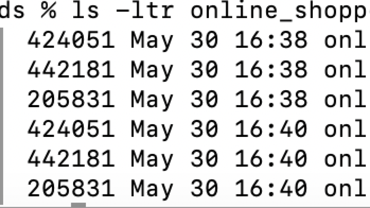
6. Next, let’s upload the online_shoppers_intentions4.csv, online_shoppers_intentions5.csv, and online_shoppers_intentions6.csv files to our S3 bucket.

We can view our files in the dataset-update-demo S3 bucket.

The dataset update job will get triggered at the specified schedule and create a new version of the dataset.

When the job is complete, dataset version 2 will have all the files from version 1 and the additional files processed by the dataset update job. In our case, version 1 has three files and the update job picked up three additional files, so the final dataset version has six files.

We can view the new version that was created on the Version history tab.

The Data tab contains a preview of the dataset and provides a list of all the files in the latest version of the dataset.

Retrain the ML model with an updated dataset

Let’s retrain our ML model with the latest version of the dataset.

1. On the My models page, choose your model.
2. Choose Add version.
   
3. Select the latest dataset version (v2 in our case) and choose Select dataset.
   
4. Keep the target column and build configuration similar to the previous model version.
   

When the training is complete, let’s evaluate the model performance. The following screenshot shows that adding additional data and retraining our ML model has helped improve our model performance.

Create a prediction dataset

With an ML model trained, let’s create a dataset for predictions and run batch predictions on it.

1. On the Datasets page, create a tabular dataset.
2. Enter a name and choose Create.
   
3. In our S3 bucket, upload one file with 500 rows to predict.
   

Next, we set up auto updates on the prediction dataset.

4. Toggle Enable auto update to on and specify the data source.
5. Select the frequency and specify a starting time.
6. Save the configuration.
   

Automate the batch prediction workflow on an auto updated predictions dataset

In this step, we configure our auto batch prediction workflows.

1. On the My models page, navigate to version 2 of your model.
2. On the Predict tab, choose Batch prediction and Automatic.
   
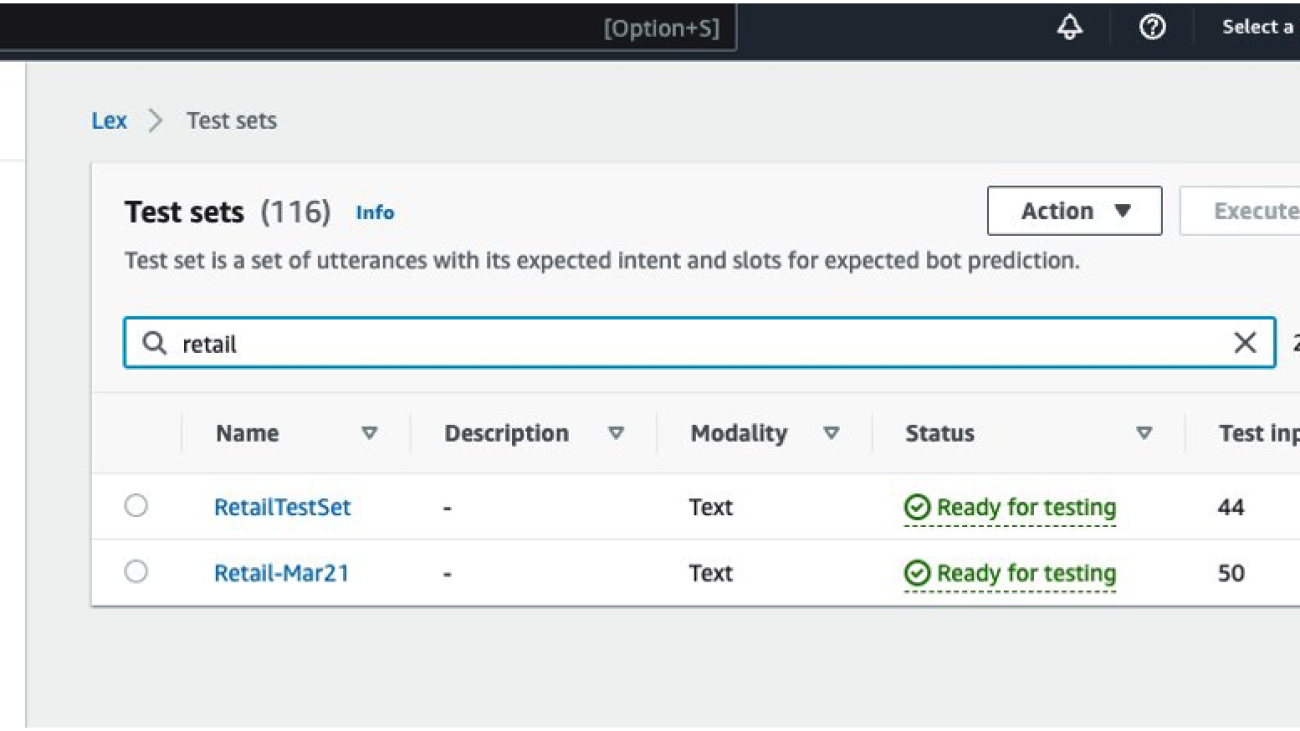
3. Choose Select dataset to specify the dataset to generate predictions on.
   
4. Select the predict dataset that we created earlier and choose Choose dataset.
   
5. Choose Set up.
   

We now have an automatic batch prediction workflow. This will be triggered when the Predict dataset is automatically updated.

Now let’s upload more CSV files to the predict S3 folder.

This operation will trigger an auto update of the predict dataset.

This will in turn trigger the automatic batch prediction workflow and generate predictions for us to view.

We can view all automations on the Automations page.

Thanks to the automatic dataset update and automatic batch prediction workflows, we can use the latest version of the tabular, image, and document dataset for training ML models, and build batch prediction workflows that get automatically triggered on every dataset update.

Clean up

To avoid incurring future charges, log out of Canvas. Canvas bills you for the duration of the session, and we recommend logging out of Canvas when you’re not using it. Refer to Logging out of Amazon SageMaker Canvas for more details.

Conclusion

In this post, we discussed how we can use the new dataset update capability to build new dataset versions and train our ML models with the latest data in Canvas. We also showed how we can efficiently automate the process of running batch predictions on updated data.

To start your low-code/no-code ML journey, refer to the Amazon SageMaker Canvas Developer Guide.

Special thanks to everyone who contributed to the launch.

About the Authors

Janisha Anand is a Senior Product Manager on the SageMaker No/Low-Code ML team, which includes SageMaker Canvas and SageMaker Autopilot. She enjoys coffee, staying active, and spending time with her family.

Prashanth is a Software Development Engineer at Amazon SageMaker and mainly works with SageMaker low-code and no-code products.

Esha Dutta is a Software Development Engineer at Amazon SageMaker. She focuses on building ML tools and products for customers. Outside of work, she enjoys the outdoors, yoga, and hiking.

Read More

Amazon Lex is excited to announce Test Workbench, a new bot testing solution that provides tools to simplify and automate the bot testing process. During bot development, testing is the phase where developers check whether a bot meets the specific requirements, needs and expectations by identifying errors, defects, or bugs in the system before scaling. Testing helps validate bot performance on several fronts such as conversational flow (understanding user queries and responding accurately), intent overlap handling, and consistency across modalities. However, testing is often manual, error-prone, and non-standardized. Test Workbench standardizes automated test management by allowing chatbot development teams to generate, maintain, and execute test sets with a consistent methodology and avoid custom scripting and ad-hoc integrations. In this post, you will learn how Test Workbench streamlines automated testing of a bot’s voice and text modalities and provides accuracy and performance measures for parameters such as audio transcription, intent recognition, and slot resolution for both single utterance inputs and multi-turn conversations. This allows you to quickly identify bot improvement areas and maintain a consistent baseline to measure accuracy over time and observe any accuracy regression due to bot updates.

Amazon Lex is a fully managed service for building conversational voice and text interfaces. Amazon Lex helps you build and deploy chatbots and virtual assistants on websites, contact center services, and messaging channels. Amazon Lex bots help increase interactive voice response (IVR) productivity, automate simple tasks, and drive operational efficiencies across the organization. Test Workbench for Amazon Lex standardizes and simplifies the bot testing lifecycle, which is critical to improving bot design.

Features of Test Workbench

Test Workbench for Amazon Lex includes the following features:

• Generate test datasets automatically from a bot’s conversation logs
• Upload manually built test set baselines
• Perform end-to-end testing of single input or multi-turn conversations
• Test both audio and text modalities of a bot
• Review aggregated and drill-down metrics for bot dimensions:
  • Speech transcription
  • Intent recognition
  • Slot resolution (including multi-valued slots or composite slots)
  • Context tags
  • Session attributes
  • Request attributes
  • Runtime hints
  • Time delay in seconds

Prerequisites

To test this feature, you should have the following:

• An AWS account with administrator access
• A sample retail bot imported via the Amazon Lex console (for more information, refer to importing a bot)
• A test set source, either from:
  • Conversation logs enabled for the bot to store bot interactions, or
  • A sample retail test set that can be imported following the instructions provided in this post

In addition, you should have knowledge and understanding of the following services and features:

• Amazon Lex
• Amazon CloudWatch
• AWS Identity and Access Management (IAM)

Create a test set

To create your test set, complete the following steps:

1. On the Amazon Lex console, under Test workbench in the navigation pane, choose Test sets.

You can review a list of existing test sets, including basic information such as name, description, number of test inputs, modality, and status. In the following steps, you can choose between generating a test set from the conversation logs associated with the bot or uploading an existing manually built test set in a CSV file format.

2. Choose Create test set.

• Generating test sets from conversation logs allows you to do the following:
  • Include real multi-turn conversations from the bot’s logs in CloudWatch
  • Include audio logs and conduct tests that account for real speech nuances, background noises, and accents
  • Speed up the creation of test sets
• Uploading a manually built test set allows you to do the following:
  • Test new bots for which there is no production data
  • Perform regression tests on existing bots for any new or modified intents, slots, and conversation flows
  • Test carefully crafted and detailed scenarios that specify session attributes and request attributes

To generate a test set, complete the following steps. To upload a manually built test set, skip to step 7.

3. Choose Generate a baseline test set.
4. Choose your options for Bot name, Bot alias, and Language.
5. For Time range, set a time range for the logs.
6. For Existing IAM role, choose a role.

Ensure that the IAM role is able to grant you access to retrieve information from the conversation logs. Refer to Creating IAM roles to create an IAM role with the appropriate policy.

7. If you prefer to use a manually created test set, select Upload a file to this test set.
8. For Upload a file to this test set, choose from the following options:
   • Select Upload from S3 bucket to upload a CSV file from an Amazon Simple Storage Service (Amazon S3) bucket.
   • Select Upload a file to this test set to upload a CSV file from your computer.

You can use the sample test set provided in this post. For more information about templates, choose the CSV Template link on the page.

9. For Modality, select the modality of your test set, either Text or Audio.

Test Workbench provides testing support for audio and text input formats.

10. For S3 location, enter the S3 bucket location where the results will be stored.
11. Optionally, choose an AWS Key Management Service (AWS KMS) key to encrypt output transcripts.
12. Choose Create.

Your newly created test set will be listed on the Test sets page with one of the following statuses:

• Ready for annotation – For test sets generated from Amazon Lex bot conversation logs, the annotation step serves as a manual gating mechanism to ensure quality test inputs. By annotating values for expected intents and expected slots for each test line item, you indicate the “ground truth” for that line. The test results from the bot run are collected and compared against the ground truth to mark test results as pass or fail. This line level comparison then allows for creating aggregated measures.
• Ready for testing – This indicates that the test set is ready to be executed against an Amazon Lex bot.
• Validation error – Uploaded test files are checked for errors such as exceeding maximum supported length, invalid characters in intent names, or invalid Amazon S3 links containing audio files. If the test set is in the Validation error state, download the file showing the validation details to see test input issues or errors on a line-by-line basis. Once they are addressed, you can manually upload the corrected test set CSV into the test set.

Executing a test set

A test set is de-coupled from a bot. The same test set can be executed against a different bot or bot alias in the future as your business use case evolves. To report performance metrics of a bot against the baseline test data, complete the following steps:

1. Import the sample bot definition and build the bot (refer to Importing a bot for guidance).
2. On the Amazon Lex console, choose Test sets in the navigation pane.
3. Choose your validated test set.

Here you can review basic information about the test set and the imported test data.

4. Choose Execute test.
   
5. Choose the appropriate options for Bot name, Bot alias, and Language.
6. For Test type, select Audio or Text.
7. For Endpoint selection, select either Streaming or Non-streaming.
8. Choose Validate discrepancy to validate your test dataset.
   

Before executing a test set, you can validate test coverage, including identifying intents and slots present in the test set but not in the bot. This early warning serves to set tester expectation for unexpected test failures. If discrepancies between your test dataset and your bot are detected, the Execute test page will update with the View details button.

Intents and slots found in the test data set but not in the bot alias are listed as shown in the following screenshots.

10. After you validate the discrepancies, choose Execute to run the test.

Review results

The performance measures generated after executing a test set help you identify areas of bot design that need improvements and are useful for expediting bot development and delivery to support your customers. Test Workbench provides insights on intent classification and slot resolution in end-to-end conversation and single-line input level. The completed test runs are stored with timestamps in your S3 bucket, and can be used for future comparative reviews.

1. On the Amazon Lex console, choose Test results in the navigation pane.
2. Choose the test result ID for the results you want to review.

On the next page, the test results will include a breakdown of results organized in four main tabs:  Overall results, Conversation results, Intent and slot results, and Detailed results.

Overall results

The Overall results tab contains three main sections:

• Test set input breakdown — A chart showing the total number of end-to-end conversations and single input utterances in the test set.
• Single input breakdown — A chart showing the number of passed or failed single inputs.
• Conversation breakdown — A chart showing the number of passed or failed multi-turn inputs.

For test sets run in audio modality, speech transcription charts are provided to show the number of passed or failed speech transcriptions on both single input and conversation types. In audio modality, a single input or multi-turn conversation could pass the speech transcription test, yet fail the overall end-to-end test. This can be caused, for instance, by a slot resolution or an intent recognition issue.

Conversation results

Test Workbench helps you drill down into conversation failures that can be attributed to specific intents or slots. The Conversation results tab is organized into three main areas, covering all intents and slots used in the test set:

• Conversation pass rates — A table used to visualize which intents and slots are responsible for possible conversation failures.
• Conversation intent failure metrics — A bar graph showing the top five worst performing intents in the test set, if any.
• Conversation slot failure metrics — A bar graph showing the top five worst performing slots in the test set, if any.

Intent and slot results

The Intent and slot results tab provides drill-down metrics for bot dimensions such as intent recognition and slot resolution.

• Intent recognition metrics — A table showing the intent recognition success rate.
• Slot resolution metrics — A table showing the slot resolution success rate, by each intent.

Detailed results

You can access a detailed report of the executed test run on the Detailed results tab. A table is displayed to show the actual transcription, output intent, and slot values in a test set. The report can be downloaded as a CSV for further analysis.

The line-level output provides insights to help improve the bot design and boost accuracy. For instance, misrecognized or missed speech inputs such as branded words can be added to custom vocabulary of an intent or as utterances under an intent.

In order to further improve conversation design, you can refer to this post, outlining best practices on using ML to create a bot that will delight your customers by accurately understanding them.

Conclusion

In this post, we presented the Test Workbench for Amazon Lex, a native capability that standardizes a chatbot automated testing process and allows developers and conversation designers to streamline and iterate quickly through bot design and development.

We look forward to hearing how you use this new functionality of Amazon Lex and welcome feedback! For any questions, bugs, or feature requests, please reach us through AWS re:Post for Amazon Lex or your AWS Support contacts.

To learn more, see Amazon Lex FAQs and the Amazon Lex V2 Developer Guide.

About the authors

Sandeep Srinivasan is a Product Manager on the Amazon Lex team. As a keen observer of human behavior, he is passionate about customer experience. He spends his waking hours at the intersection of people, technology, and the future.

Grazia Russo Lassner is a Senior Consultant with the AWS Professional Services Natural Language AI team. She specializes in designing and developing conversational AI solutions using AWS technologies for customers in various industries. Outside of work, she enjoys beach weekends, reading the latest fiction books, and family.

Read More

Amazon Textract is a machine learning (ML) service that automatically extracts text, handwriting, and data from any document or image. Amazon Textract has a Tables feature within the AnalyzeDocument API that offers the ability to automatically extract tabular structures from any document. In this post, we discuss the improvements made to the Tables feature and how it makes it easier to extract information in tabular structures from a wide variety of documents.

Tabular structures in documents such as financial reports, paystubs, and certificate of analysis files are often formatted in a way that enables easy interpretation of information. They often also include information such as table title, table footer, section title, and summary rows within the tabular structure for better readability and organization. For a similar document prior to this enhancement, the Tables feature within AnalyzeDocument would have identified those elements as cells, and it didn’t extract titles and footers that are present outside the bounds of the table. In such cases, custom postprocessing logic to identify such information or extract it separately from the API’s JSON output was necessary. With this announcement of enhancements to the Table feature, the extraction of various aspects of tabular data becomes much simpler.

In April 2023, Amazon Textract introduced the ability to automatically detect titles, footers, section titles, and summary rows present in documents via the Tables feature. In this post, we discuss these enhancements and give examples to help you understand and use them in your document processing workflows. We walk through how to use these improvements through code examples to use the API and process the response with the Amazon Textract Textractor library.

Overview of solution

The following image shows that the updated model not only identifies the table in the document but all corresponding table headers and footers. This sample financial report document contains table title, footer, section title, and summary rows.

The Tables feature enhancement adds support for four new elements in the API response that allows you to extract each of these table elements with ease, and adds the ability to distinguish the type of table.

Table elements

Amazon Textract can identify several components of a table such as table cells and merged cells. These components, known as Blockobjects, encapsulate the details related to the component, such as the bounding geometry, relationships, and confidence score. A Block represents items that are recognized in a document within a group of pixels close to each other. The following are the new Table Blocks introduced in this enhancement:

• Table title – A new Block type called TABLE_TITLE that enables you to identify the title of a given table. Titles can be one or more lines, which are typically above a table or embedded as a cell within the table.
• Table footers – A new Block type called TABLE_FOOTER that enables you to identify the footers associated with a given table. Footers can be one or more lines that are typically below the table or embedded as a cell within the table.
• Section title – A new Block type called TABLE_SECTION_TITLE that enables you to identify if the cell detected is a section title.
• Summary cells – A new Block type called TABLE_SUMMARY that enables you to identify if the cell is a summary cell, such as a cell for totals on a paystub.

Types of tables

When Amazon Textract identifies a table in a document, it extracts all the details of the table into a top-level Block type of TABLE. Tables can come in various shapes and sizes. For example, documents often contain tables that may or may not have a discernible table header. To help distinguish these types of tables, we added two new entity types for a TABLE Block: SEMI_STRUCTURED_TABLE and STRUCTURED_TABLE. These entity types help you distinguish between a structured versus a semistructured table.

Structured tables are tables that have clearly defined column headers. But with semi-structured tables, data might not follow a strict structure. For example, data may appear in tabular structure that isn’t a table with defined headers. The new entity types offer the flexibility to choose which tables to keep or remove during post-processing. The following image shows an example of STRUCTURED_TABLE and SEMI_STRUCTURED_TABLE.

Analyzing the API output

In this section, we explore how you can use the Amazon Textract Textractor library to postprocess the API output of AnalyzeDocument with the Tables feature enhancements. This allows you to extract relevant information from tables.

Textractor is a library created to work seamlessly with Amazon Textract APIs and utilities to subsequently convert the JSON responses returned by the APIs into programmable objects. You can also use it to visualize entities on the document and export the data in formats such as comma-separated values (CSV) files. It’s intended to aid Amazon Textract customers in setting up their postprocessing pipelines.

In our examples, we use the following sample page from a 10-K SEC filing document.

The following code can be found within our GitHub repository. To process this document, we make use of the Textractor library and import it for us to postprocess the API outputs and visualize the data:

pip install amazon-textract-textractor

The first step is to call Amazon Textract AnalyzeDocument with Tables feature, denoted by the features=[TextractFeatures.TABLES] parameter to extract the table information. Note that this method invokes the real-time (or synchronous) AnalyzeDocument API, which supports single-page documents. However, you can use the asynchronous StartDocumentAnalysis API to process multi-page documents (with up to 3,000 pages).

from PIL import Image
from textractor import Textractor
from textractor.visualizers.entitylist import EntityList
from textractor.data.constants import TextractFeatures, Direction, DirectionalFinderType
image = Image.open("sec_filing.png") # loads the document image with Pillow
extractor = Textractor(region_name="us-east-1") # Initialize textractor client, modify region if required
document = extractor.analyze_document(
    file_source=image,
    features=[TextractFeatures.TABLES],
    save_image=True
)

The document object contains metadata about the document that can be reviewed. Notice that it recognizes one table in the document along with other entities in the document:

This document holds the following data:
Pages - 1
Words - 658
Lines - 122
Key-values - 0
Checkboxes - 0
Tables - 1
Queries - 0
Signatures - 0
Identity Documents - 0
Expense Documents – 0

Now that we have the API output containing the table information, we visualize the different elements of the table using the response structure discussed previously:

table = EntityList(document.tables[0])
document.tables[0].visualize()

The Textractor library highlights the various entities within the detected table with a different color code for each table element. Let’s dive deeper into how we can extract each element. The following code snippet demonstrates extracting the title of the table:

table_title = table[0].title.text
table_title

'The following table summarizes, by major security type, our cash, cash equivalents, restricted cash, and marketable securities that are measured at fair value on a recurring basis and are categorized using the fair value hierarchy (in millions):'

Similarly, we can use the following code to extract the footers of the table. Notice that table_footers is a list, which means that there can be one or more footers associated with the table. We can iterate over this list to see all the footers present, and as shown in the following code snippet, the output displays three footers:

table_footers = table[0].footers
for footers in table_footers:
    print (footers.text)

(1) The related unrealized gain (loss) recorded in "Other income (expense), net" was $(116) million and $1.0 billion in Q3 2021 and Q3 2022, and $6 million and $(11.3) billion for the nine months ended September 30, 2021 and 2022.

(2) We are required to pledge or otherwise restrict a portion of our cash, cash equivalents, and marketable fixed income securities primarily as collateral for real estate, amounts due to third-party sellers in certain jurisdictions, debt, and standby and trade letters of credit. We classify cash, cash equivalents, and marketable fixed income securities with use restrictions of less than twelve months as "Accounts receivable, net and other" and of twelve months or longer as non-current "Other assets" on our consolidated balance sheets. See "Note 4 - Commitments and Contingencies."

(3) Our equity investment in Rivian had a fair value of $15.6 billion and $5.2 billion as of December 31, 2021 and September 30, 2022, respectively. The investment was subject to regulatory sales restrictions resulting in a discount for lack of marketability of approximately $800 million as of December 31, 2021, which expired in Q1 2022.

Generating data for downstream ingestion

The Textractor library also helps you simplify the ingestion of table data into downstream systems or other workflows. For example, you can export the extracted table data into a human readable Microsoft Excel file. At the time of this writing, this is the only format that supports merged tables.

table[0].to_excel(filepath="sec_filing.xlsx")

We can also convert it to a Pandas DataFrame. DataFrame is a popular choice for data manipulation, analysis, and visualization in programming languages such as Python and R.

In Python, DataFrame is a primary data structure in the Pandas library. It’s flexible and powerful, and is often the first choice for data analysis professionals for various data analysis and ML tasks. The following code snippet shows how to convert the extracted table information into a DataFrame with a single line of code:

df=table[0].to_pandas()
df

Lastly, we can convert the table data into a CSV file. CSV files are often used to ingest data into relational databases or data warehouses. See the following code:

table[0].to_csv()

',0,1,2,3,4,5n0,,"December 31, 2021",,September,"30, 2022",n1,,Total Estimated Fair Value,Cost or Amortized Cost,Gross Unrealized Gains,Gross Unrealized Losses,Total Estimated Fair Valuen2,Cash,"$ 10,942","$ 10,720",$ -,$ -,"$ 10,720"n3,Level 1 securities:,,,,,n4,Money market funds,"20,312","16,697",-,-,"16,697"n5,Equity securities (1)(3),"1,646",,,,"5,988"n6,Level 2 securities:,,,,,n7,Foreign government and agency securities,181,141,-,(2),139n8,U.S. government and agency securities,"4,300","2,301",-,(169),"2,132"n9,Corporate debt securities,"35,764","20,229",-,(799),"19,430"n10,Asset-backed securities,"6,738","3,578",-,(191),"3,387"n11,Other fixed income securities,686,403,-,(22),381n12,Equity securities (1)(3),"15,740",,,,19n13,,"$ 96,309","$ 54,069",$ -,"$ (1,183)","$ 58,893"n14,"Less: Restricted cash, cash equivalents, and marketable securities (2)",(260),,,,(231)n15,"Total cash, cash equivalents, and marketable securities","$ 96,049",,,,"$ 58,662"n'</p><h2> </h2>

Conclusion

The introduction of these new block and entity types (TABLE_TITLE, TABLE_FOOTER, STRUCTURED_TABLE, SEMI_STRUCTURED_TABLE, TABLE_SECTION_TITLE, TABLE_FOOTER, and TABLE_SUMMARY) marks a significant advancement in extraction of tabular structures from documents with Amazon Textract.

These tools provide a more nuanced and flexible approach, catering to both structured and semistructured tables and making sure that no important data is overlooked, regardless of its location in a document.

This means we can now handle diverse data types and table structures with enhanced efficiency and accuracy. As we continue to embrace the power of automation in document processing workflows, these enhancements will no doubt pave the way for more streamlined workflows, higher productivity, and more insightful data analysis. For more information on AnalyzeDocument and the Tables feature, refer to AnalyzeDocument.

About the authors

Raj Pathak is a Senior Solutions Architect and Technologist specializing in Financial Services (Insurance, Banking, Capital Markets) and Machine Learning. He specializes in Natural Language Processing (NLP), Large Language Models (LLM) and Machine Learning infrastructure and operations projects (MLOps).

Anjan Biswas is a Senior AI Services Solutions Architect with focus on AI/ML and Data Analytics. Anjan is part of the world-wide AI services team and works with customers to help them understand, and develop solutions to business problems with AI and ML. Anjan has over 14 years of experience working with global supply chain, manufacturing, and retail organizations and is actively helping customers get started and scale on AWS AI services.

Lalita Reddi is a Senior Technical Product Manager with the Amazon Textract team. She is focused on building machine learning-based services for AWS customers. In her spare time, Lalita likes to play board games, and go on hikes.

Read More