Monthly Archives: September 2023

Machine learning (ML) is becoming increasingly complex as customers try to solve more and more challenging problems. This complexity often leads to the need for distributed ML, where multiple machines are used to train a single model. Although this enables parallelization of tasks across multiple nodes, leading to accelerated training times, enhanced scalability, and improved performance, there are significant challenges in effectively using distributed hardware. Data scientists have to address challenges like data partitioning, load balancing, fault tolerance, and scalability. ML engineers must handle parallelization, scheduling, faults, and retries manually, requiring complex infrastructure code.

In this post, we discuss the benefits of using Ray and Amazon SageMaker for distributed ML, and provide a step-by-step guide on how to use these frameworks to build and deploy a scalable ML workflow.

Ray, an open-source distributed computing framework, provides a flexible framework for distributed training and serving of ML models. It abstracts away low-level distributed system details through simple, scalable libraries for common ML tasks such as data preprocessing, distributed training, hyperparameter tuning, reinforcement learning, and model serving.

SageMaker is a fully managed service for building, training, and deploying ML models. Ray seamlessly integrates with SageMaker features to build and deploy complex ML workloads that are both efficient and reliable. The combination of Ray and SageMaker provides end-to-end capabilities for scalable ML workflows, and has the following highlighted features:

• Distributed actors and parallelism constructs in Ray simplify developing distributed applications.
• Ray AI Runtime (AIR) reduces friction of going from development to production. With Ray and AIR, the same Python code can scale seamlessly from a laptop to a large cluster.
• The managed infrastructure of SageMaker and features like processing jobs, training jobs, and hyperparameter tuning jobs can use Ray libraries underneath for distributed computing.
• Amazon SageMaker Experiments allows rapidly iterating and keeping track of trials.
• Amazon SageMaker Feature Store provides a scalable repository for storing, retrieving, and sharing ML features for model training.
• Trained models can be stored, versioned, and tracked in Amazon SageMaker Model Registry for governance and management.

• Amazon SageMaker Pipelines allows orchestrating the end-to-end ML lifecycle from data preparation and training to model deployment as automated workflows.

Solution overview

This post focuses on the benefits of using Ray and SageMaker together. We set up an end-to-end Ray-based ML workflow, orchestrated using SageMaker Pipelines. The workflow includes parallel ingestion of data into the feature store using Ray actors, data preprocessing with Ray Data, training models and hyperparameter tuning at scale using Ray Train and hyperparameter optimization (HPO) tuning jobs, and finally model evaluation and registering the model into a model registry.

For our data, we use a synthetic housing dataset that consists of eight features (YEAR_BUILT, SQUARE_FEET, NUM_BEDROOM, NUM_BATHROOMS, LOT_ACRES, GARAGE_SPACES, FRONT_PORCH, and DECK) and our model will predict the PRICE of the house.

Each stage in the ML workflow is broken into discrete steps, with its own script that takes input and output parameters. In the next section, we highlight key code snippets from each step. The full code can be found on the aws-samples-for-ray GitHub repository.

Prerequisites

To use the SageMaker Python SDK and run the code associated with this post, you need the following prerequisites:

• An AWS account that contains all your AWS resources
• An AWS Identity and Access Management (IAM) role with access to Amazon SageMaker Studio notebooks, SageMaker Feature Store, SageMaker Model Registry, and SageMaker Pipelines

Ingest data into SageMaker Feature Store

The first step in the ML workflow is to read the source data file from Amazon Simple Storage Service (Amazon S3) in CSV format and ingest it into SageMaker Feature Store. SageMaker Feature Store is a purpose-built repository that makes it easy for teams to create, share, and manage ML features. It simplifies feature discovery, reuse, and sharing, leading to faster development, increased collaboration within customer teams, and reduced costs.

Ingesting features into the feature store contains the following steps:

1. Define a feature group and create the feature group in the feature store.
2. Prepare the source data for the feature store by adding an event time and record ID for each row of data.
3. Ingest the prepared data into the feature group by using the Boto3 SDK.

In this section, we only highlight Step 3, because this is the part that involves parallel processing of the ingestion task using Ray. You can review the full code for this process in the GitHub repo.

The ingest_features method is defined inside a class called Featurestore. Note that the Featurestore class is decorated with @ray.remote. This indicates that an instance of this class is a Ray actor, a stateful and concurrent computational unit within Ray. It’s a programming model that allows you to create distributed objects that maintain an internal state and can be accessed concurrently by multiple tasks running on different nodes in a Ray cluster. Actors provide a way to manage and encapsulate the mutable state, making them valuable for building complex, stateful applications in a distributed setting. You can specify resource requirements in actors too. In this case, each instance of the FeatureStore class will require 0.5 CPUs. See the following code:

@ray.remote(num_cpus=0.5)
class Featurestore:
    def ingest_features(self,feature_group_name, df, region):
        """
        Ingest features to Feature Store Group
        Args:
            feature_group_name (str): Feature Group Name
            data_path (str): Path to the train/validation/test data in CSV format.
        """
        
        ...

You can interact with the actor by calling the remote operator. In the following code, the desired number of actors is passed in as an input argument to the script. The data is then partitioned based on the number of actors and passed to the remote parallel processes to be ingested into the feature store. You can call get on the object ref to block the execution of the current task until the remote computation is complete and the result is available. When the result is available, ray.get will return the result, and the execution of the current task will continue.

import modin.pandas as pd
import ray

df = pd.read_csv(s3_path)
data = prepare_df_for_feature_store(df)
# Split into partitions
partitions = [ray.put(part) for part in np.array_split(data, num_actors)]
# Start actors and assign partitions in a loop
actors = [Featurestore.remote() for _ in range(args.num_actors)]
results = []

for actor, partition in zip(actors, input_partitions):
    results.append(actor.ingest_features.remote(
                        args.feature_group_name, 
                        partition, args.region
                      )
                )

ray.get(results)

Prepare data for training, validation, and testing

In this step, we use Ray Dataset to efficiently split, transform, and scale our dataset in preparation for machine learning. Ray Dataset provides a standard way to load distributed data into Ray, supporting various storage systems and file formats. It has APIs for common ML data preprocessing operations like parallel transformations, shuffling, grouping, and aggregations. Ray Dataset also handles operations needing stateful setup and GPU acceleration. It integrates smoothly with other data processing libraries like Spark, Pandas, NumPy, and more, as well as ML frameworks like TensorFlow and PyTorch. This allows building end-to-end data pipelines and ML workflows on top of Ray. The goal is to make distributed data processing and ML easier for practitioners and researchers.

Let’s look at sections of the scripts that perform this data preprocessing. We start by loading the data from the feature store:

def load_dataset(feature_group_name, region):
    """
    Loads the data as a ray dataset from the offline featurestore S3 location
    Args:
        feature_group_name (str): name of the feature group
    Returns:
        ds (ray.data.dataset): Ray dataset the contains the requested dat from the feature store
    """
    session = sagemaker.Session(boto3.Session(region_name=region))
    fs_group = FeatureGroup(
        name=feature_group_name, 
        sagemaker_session=session
    )

    fs_data_loc = fs_group.describe().get("OfflineStoreConfig").get("S3StorageConfig").get("ResolvedOutputS3Uri")
    
    # Drop columns added by the feature store
    # Since these are not related to the ML problem at hand
    cols_to_drop = ["record_id", "event_time","write_time", 
                    "api_invocation_time", "is_deleted", 
                    "year", "month", "day", "hour"]           

    ds = ray.data.read_parquet(fs_data_loc)
    ds = ds.drop_columns(cols_to_drop)
    print(f"{fs_data_loc} count is {ds.count()}")
    return ds

We then split and scale data using the higher-level abstractions available from the ray.data library:

def split_dataset(dataset, train_size, val_size, test_size, random_state=None):
    """
    Split dataset into train, validation and test samples
    Args:
        dataset (ray.data.Dataset): input data
        train_size (float): ratio of data to use as training dataset
        val_size (float): ratio of data to use as validation dataset
        test_size (float): ratio of data to use as test dataset
        random_state (int): Pass an int for reproducible output across multiple function calls.
    Returns:
        train_set (ray.data.Dataset): train dataset
        val_set (ray.data.Dataset): validation dataset
        test_set (ray.data.Dataset): test dataset
    """
    # Shuffle this dataset with a fixed random seed.
    shuffled_ds = dataset.random_shuffle(seed=random_state)
    # Split the data into train, validation and test datasets
    train_set, val_set, test_set = shuffled_ds.split_proportionately([train_size, val_size])
    return train_set, val_set, test_set

def scale_dataset(train_set, val_set, test_set, target_col):
    """
    Fit StandardScaler to train_set and apply it to val_set and test_set
    Args:
        train_set (ray.data.Dataset): train dataset
        val_set (ray.data.Dataset): validation dataset
        test_set (ray.data.Dataset): test dataset
        target_col (str): target col
    Returns:
        train_transformed (ray.data.Dataset): train data scaled
        val_transformed (ray.data.Dataset): val data scaled
        test_transformed (ray.data.Dataset): test data scaled
    """
    tranform_cols = dataset.columns()
    # Remove the target columns from being scaled
    tranform_cols.remove(target_col)
    # set up a standard scaler
    standard_scaler = StandardScaler(tranform_cols)
    # fit scaler to training dataset
    print("Fitting scaling to training data and transforming dataset...")
    train_set_transformed = standard_scaler.fit_transform(train_set)
    # apply scaler to validation and test datasets
    print("Transforming validation and test datasets...")
    val_set_transformed = standard_scaler.transform(val_set)
    test_set_transformed = standard_scaler.transform(test_set)
    return train_set_transformed, val_set_transformed, test_set_transformed

The processed train, validation, and test datasets are stored in Amazon S3 and will be passed as the input parameters to subsequent steps.

Perform model training and hyperparameter optimization

With our data preprocessed and ready for modeling, it’s time to train some ML models and fine-tune their hyperparameters to maximize predictive performance. We use XGBoost-Ray, a distributed backend for XGBoost built on Ray that enables training XGBoost models on large datasets by using multiple nodes and GPUs. It provides simple drop-in replacements for XGBoost’s train and predict APIs while handling the complexities of distributed data management and training under the hood.

To enable distribution of the training over multiple nodes, we utilize a helper class named RayHelper. As shown in the following code, we use the resource configuration of the training job and choose the first host as the head node:

class RayHelper():
    def __init__(self, ray_port:str="9339", redis_pass:str="redis_password"):
        ....
        self.resource_config = self.get_resource_config()
        self.head_host = self.resource_config["hosts"][0]
        self.n_hosts = len(self.resource_config["hosts"])

We can use the host information to decide how to initialize Ray on each of the training job instances:

def start_ray(self): 
   head_ip = self._get_ip_from_host()
   # If the current host is the host choosen as the head node
   # run `ray start` with specifying the --head flag making this is the head node
    if self.resource_config["current_host"] == self.head_host:
        output = subprocess.run(['ray', 'start', '--head', '-vvv', '--port', 
        self.ray_port, '--redis-password', self.redis_pass, 
        '--include-dashboard', 'false'], stdout=subprocess.PIPE)
        print(output.stdout.decode("utf-8"))
        ray.init(address="auto", include_dashboard=False)
        self._wait_for_workers()
        print("All workers present and accounted for")
        print(ray.cluster_resources())

    else:
       # If the current host is not the head node, 
       # run `ray start` with specifying ip address as the head_host as the head node
        time.sleep(10)
        output = subprocess.run(['ray', 'start', 
        f"--address={head_ip}:{self.ray_port}", 
        '--redis-password', self.redis_pass, "--block"], stdout=subprocess.PIPE)
        print(output.stdout.decode("utf-8"))
        sys.exit(0)

When a training job is started, a Ray cluster can be initialized by calling the start_ray() method on an instance of RayHelper:

if __name__ == '__main__':
    ray_helper = RayHelper()
    ray_helper.start_ray()
    args = read_parameters()
    sess = sagemaker.Session(boto3.Session(region_name=args.region))

We then use the XGBoost trainer from XGBoost-Ray for training:

def train_xgboost(ds_train, ds_val, params, num_workers, target_col = "price") -> Result:
    """
    Creates a XGBoost trainer, train it, and return the result.        
    Args:
        ds_train (ray.data.dataset): Training dataset
        ds_val (ray.data.dataset): Validation dataset
        params (dict): Hyperparameters
        num_workers (int): number of workers to distribute the training across
        target_col (str): target column
    Returns:
        result (ray.air.result.Result): Result of the training job
    """
    
    train_set = RayDMatrix(ds_train, 'PRICE')
    val_set = RayDMatrix(ds_val, 'PRICE')
    
    evals_result = {}
    
    trainer = train(
        params=params,
        dtrain=train_set,
        evals_result=evals_result,
        evals=[(val_set, "validation")],
        verbose_eval=False,
        num_boost_round=100,
        ray_params=RayParams(num_actors=num_workers, cpus_per_actor=1),
    )
    
    output_path=os.path.join(args.model_dir, 'model.xgb')
    
    trainer.save_model(output_path)
    
    valMAE = evals_result["validation"]["mae"][-1]
    valRMSE = evals_result["validation"]["rmse"][-1]
 
    print('[3] #011validation-mae:{}'.format(valMAE))
    print('[4] #011validation-rmse:{}'.format(valRMSE))
    
    local_testing = False
    try:
        load_run(sagemaker_session=sess)
    except:
        local_testing = True
    if not local_testing: # Track experiment if using SageMaker Training
        with load_run(sagemaker_session=sess) as run:
            run.log_metric('validation-mae', valMAE)
            run.log_metric('validation-rmse', valRMSE)

Note that while instantiating the trainer, we pass RayParams, which takes the number actors and number of CPUs per actors. XGBoost-Ray uses this information to distribute the training across all the nodes attached to the Ray cluster.

We now create a XGBoost estimator object based on the SageMaker Python SDK and use that for the HPO job.

Orchestrate the preceding steps using SageMaker Pipelines

To build an end-to-end scalable and reusable ML workflow, we need to use a CI/CD tool to orchestrate the preceding steps into a pipeline. SageMaker Pipelines has direct integration with SageMaker, the SageMaker Python SDK, and SageMaker Studio. This integration allows you to create ML workflows with an easy-to-use Python SDK, and then visualize and manage your workflow using SageMaker Studio. You can also track the history of your data within the pipeline execution and designate steps for caching.

SageMaker Pipelines creates a Directed Acyclic Graph (DAG) that includes steps needed to build an ML workflow. Each pipeline is a series of interconnected steps orchestrated by data dependencies between steps, and can be parameterized, allowing you to provide input variables as parameters for each run of the pipeline. SageMaker Pipelines has four types of pipeline parameters: ParameterString, ParameterInteger, ParameterFloat, and ParameterBoolean. In this section, we parameterize some of the input variables and set up the step caching configuration:

processing_instance_count = ParameterInteger(
    name='ProcessingInstanceCount',
    default_value=1
)
feature_group_name = ParameterString(
    name='FeatureGroupName',
    default_value='fs-ray-synthetic-housing-data'
)
bucket_prefix = ParameterString(
    name='Bucket_Prefix',
    default_value='aws-ray-mlops-workshop/feature-store'
)
rmse_threshold = ParameterFloat(name="RMSEThreshold", default_value=15000.0)
    train_size = ParameterString(
    name='TrainSize',
    default_value="0.6"
)
val_size = ParameterString(
    name='ValidationSize',
    default_value="0.2"
)
test_size = ParameterString(
    name='TestSize',
    default_value="0.2"
)

cache_config = CacheConfig(enable_caching=True, expire_after="PT12H")

We define two processing steps: one for SageMaker Feature Store ingestion, the other for data preparation. This should look very similar to the previous steps described earlier. The only new line of code is the ProcessingStep after the steps’ definition, which allows us to take the processing job configuration and include it as a pipeline step. We further specify the dependency of the data preparation step on the SageMaker Feature Store ingestion step. See the following code:

feature_store_ingestion_step = ProcessingStep(
    name='FeatureStoreIngestion',
    step_args=fs_processor_args,
    cache_config=cache_config
)

preprocess_dataset_step = ProcessingStep(
    name='PreprocessData',
    step_args=processor_args,
    cache_config=cache_config
)
preprocess_dataset_step.add_depends_on([feature_store_ingestion_step])

Similarly, to build a model training and tuning step, we need to add a definition of TuningStep after the model training step’s code to allow us to run SageMaker hyperparameter tuning as a step in the pipeline:

tuning_step = TuningStep(
    name="HPTuning",
    tuner=tuner,
    inputs={
        "train": TrainingInput(
            s3_data=preprocess_dataset_step.properties.ProcessingOutputConfig.Outputs[
            "train"
            ].S3Output.S3Uri,
            content_type="text/csv"
        ),
        "validation": TrainingInput(
            s3_data=preprocess_dataset_step.properties.ProcessingOutputConfig.Outputs[
            "validation"
            ].S3Output.S3Uri,
            content_type="text/csv"
        )
    },
    cache_config=cache_config,
)
tuning_step.add_depends_on([preprocess_dataset_step])

After the tuning step, we choose to register the best model into SageMaker Model Registry. To control the model quality, we implement a minimum quality gate that compares the best model’s objective metric (RMSE) against a threshold defined as the pipeline’s input parameter rmse_threshold. To do this evaluation, we create another processing step to run an evaluation script. The model evaluation result will be stored as a property file. Property files are particularly useful when analyzing the results of a processing step to decide how other steps should be run. See the following code:

# Specify where we'll store the model evaluation results so that other steps can access those results
evaluation_report = PropertyFile(
    name='EvaluationReport',
    output_name='evaluation',
    path='evaluation.json',
)

# A ProcessingStep is used to evaluate the performance of a selected model from the HPO step. 
# In this case, the top performing model is evaluated. 
evaluation_step = ProcessingStep(
    name='EvaluateModel',
    processor=evaluation_processor,
    inputs=[
        ProcessingInput(
            source=tuning_step.get_top_model_s3_uri(
                top_k=0, s3_bucket=bucket, prefix=s3_prefix
            ),
            destination='/opt/ml/processing/model',
        ),
        ProcessingInput(
            source=preprocess_dataset_step.properties.ProcessingOutputConfig.Outputs['test'].S3Output.S3Uri,
            destination='/opt/ml/processing/test',
        ),
    ],
    outputs=[
        ProcessingOutput(
            output_name='evaluation', source='/opt/ml/processing/evaluation'
        ),
    ],
    code='./pipeline_scripts/evaluate/script.py',
    property_files=[evaluation_report],
)

We define a ModelStep to register the best model into SageMaker Model Registry in our pipeline. In case the best model doesn’t pass our predetermined quality check, we additionally specify a FailStep to output an error message:

register_step = ModelStep(
    name='RegisterTrainedModel',
    step_args=model_registry_args
)

metrics_fail_step = FailStep(
    name="RMSEFail",
    error_message=Join(on=" ", values=["Execution failed due to RMSE >", rmse_threshold]),
)

Next, we use a ConditionStep to evaluate whether the model registration step or failure step should be taken next in the pipeline. In our case, the best model will be registered if its RMSE score is lower than the threshold.

# Condition step for evaluating model quality and branching execution
cond_lte = ConditionLessThanOrEqualTo(
    left=JsonGet(
        step_name=evaluation_step.name,
        property_file=evaluation_report,
        json_path='regression_metrics.rmse.value',
    ),
    right=rmse_threshold,
)
condition_step = ConditionStep(
    name='CheckEvaluation',
    conditions=[cond_lte],
    if_steps=[register_step],
    else_steps=[metrics_fail_step],
)

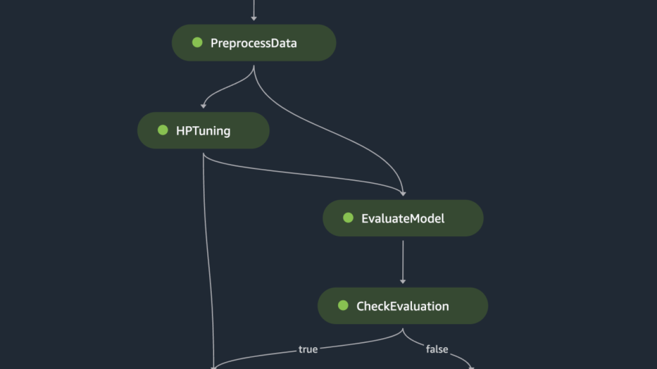
Finally, we orchestrate all the defined steps into a pipeline:

pipeline_name = 'synthetic-housing-training-sm-pipeline-ray'
step_list = [
             feature_store_ingestion_step,
             preprocess_dataset_step,
             tuning_step,
             evaluation_step,
             condition_step
            ]

training_pipeline = Pipeline(
    name=pipeline_name,
    parameters=[
        processing_instance_count,
        feature_group_name,
        train_size,
        val_size,
        test_size,
        bucket_prefix,
        rmse_threshold
    ],
    steps=step_list
)

# Note: If an existing pipeline has the same name it will be overwritten.
training_pipeline.upsert(role_arn=role_arn)

The preceding pipeline can be visualized and executed directly in SageMaker Studio, or be executed by calling execution = training_pipeline.start(). The following figure illustrates the pipeline flow.

Additionally, we can review the lineage of artifacts generated by the pipeline execution.

from sagemaker.lineage.visualizer import LineageTableVisualizer

viz = LineageTableVisualizer(sagemaker.session.Session())
for execution_step in reversed(execution.list_steps()):
    print(execution_step)
    display(viz.show(pipeline_execution_step=execution_step))
    time.sleep(5)

Deploy the model

After the best model is registered in SageMaker Model Registry via a pipeline run, we deploy the model to a real-time endpoint by using the fully managed model deployment capabilities of SageMaker. SageMaker has other model deployment options to meet the needs of different use cases. For details, refer to Deploy models for inference when choosing the right option for your use case. First, let’s get the model registered in SageMaker Model Registry:

xgb_regressor_model = ModelPackage(
    role_arn,
    model_package_arn=model_package_arn,
    name=model_name
)

The model’s current status is PendingApproval. We need to set its status to Approved prior to deployment:

sagemaker_client.update_model_package(
    ModelPackageArn=xgb_regressor_model.model_package_arn,
    ModelApprovalStatus='Approved'
)

xgb_regressor_model.deploy(
    initial_instance_count=1,
    instance_type='ml.m5.xlarge',
    endpoint_name=endpoint_name
)

Clean up

After you are done experimenting, remember to clean up the resources to avoid unnecessary charges. To clean up, delete the real-time endpoint, model group, pipeline, and feature group by calling the APIs DeleteEndpoint, DeleteModelPackageGroup, DeletePipeline, and DeleteFeatureGroup, respectively, and shut down all SageMaker Studio notebook instances.

Conclusion

This post demonstrated a step-by-step walkthrough on how to use SageMaker Pipelines to orchestrate Ray-based ML workflows. We also demonstrated the capability of SageMaker Pipelines to integrate with third-party ML tools. There are various AWS services that support Ray workloads in a scalable and secure fashion to ensure performance excellence and operational efficiency. Now, it’s your turn to explore these powerful capabilities and start optimizing your machine learning workflows with Amazon SageMaker Pipelines and Ray. Take action today and unlock the full potential of your ML projects!

About the Author

Raju Rangan is a Senior Solutions Architect at Amazon Web Services (AWS). He works with government sponsored entities, helping them build AI/ML solutions using AWS. When not tinkering with cloud solutions, you’ll catch him hanging out with family or smashing birdies in a lively game of badminton with friends.

Sherry Ding is a senior AI/ML specialist solutions architect at Amazon Web Services (AWS). She has extensive experience in machine learning with a PhD degree in computer science. She mainly works with public sector customers on various AI/ML-related business challenges, helping them accelerate their machine learning journey on the AWS Cloud. When not helping customers, she enjoys outdoor activities.

Read More

This post is co-authored with Richard Alexander and Mark Hallows from Arup.

Arup is a global collective of designers, consultants, and experts dedicated to sustainable development. Data underpins Arup consultancy for clients with world-class collection and analysis providing insight to make an impact.

The solution presented here is to direct decision-making processes for resilient city design. Informing design decisions towards more sustainable choices reduces the overall urban heat islands (UHI) effect and improves quality of life metrics for air quality, water quality, urban acoustics, biodiversity, and thermal comfort. Identifying key areas within an urban environment for intervention allows Arup to provide the best guidance in the industry and create better quality of life for citizens around the planet.

Urban heat islands describe the effect urban areas have on temperature compared to surrounding rural environments. Understanding how UHI affects our cities leads to improved designs that reduce the impact of urban heat on residents. The UHI effect impacts human health, greenhouse gas emissions, and water quality, and leads to increased energy usage. For city authorities, asset owners, and developers, understanding the impact on the population is key to improving quality of life and natural ecosystems. Modeling UHI accurately is a complex challenge, which Arup is now solving with earth observation data and Amazon SageMaker.

This post shows how Arup partnered with AWS to perform earth observation analysis with Amazon SageMaker geospatial capabilities to unlock UHI insights from satellite imagery. SageMaker geospatial capabilities make it easy for data scientists and machine learning (ML) engineers to build, train, and deploy models using geospatial data. SageMaker geospatial capabilities allow you to efficiently transform and enrich large-scale geospatial datasets, accelerate product development and time to insight with pre-trained ML models, and explore model predictions and geospatial data on an interactive map using 3D accelerated graphics and built-in visualization tools.

Overview of solution

The initial solution focuses on London, where during a heatwave in the summer of 2022, the UK Health Security Agency estimated 2,803 excess deaths were caused due to heat. Identifying areas within an urban environment where people may be more vulnerable to the UHI effect allows public services to direct assistance where it will have the greatest impact. This can even be forecast prior to high temperature events, reducing the impact of extreme weather and delivering a positive outcome for city dwellers.

Earth Observation (EO) data was used to perform the analysis at city scale. However, the total size poses challenges with traditional ways of storing, organizing, and querying data for large geographical areas. Arup addressed this challenge by partnering with AWS and using SageMaker geospatial capabilities to enable analysis at a city scale and beyond. As the geographic area grows to larger metropolitan areas like Los Angeles or Tokyo, the more storage and compute for analysis is required. The elasticity of AWS infrastructure is ideal for UHI analyses of urban environments of any size.

The solution: UHeat

Arup used SageMaker to develop UHeat, a digital solution that analyzes huge areas of cities to identify particular buildings, structures, and materials that are causing temperatures to rise. UHeat uses a combination of satellite imagery and open-source climate data to perform the analysis.

A small team at Arup undertook the initial analysis, during which additional data scientists needed to be trained on the SageMaker tooling and workflows. Onboarding data scientists to a new project used to take weeks using in-house tools. This now takes a matter of hours with SageMaker.

The first step of any EO analysis is the collection and preparation of the data. With SageMaker, Arup can access data from a catalog of geospatial data providers, including Sentinel-2 data, which was used for the London analysis. Built-in geospatial dataset access saves weeks of effort otherwise lost to collecting and preparing data from various data providers and vendors. EO imagery is frequently made up of small tiles which, to cover an area the size of London, need to be combined. This is known as a geomosaic, which can be created automatically using the managed geospatial operations in a SageMaker Geomosaic Earth Observation job.

After the EO data for the area of interest is compiled, the key influencing parameters for the analysis can be extracted. For UHI, Arup needed to be able to derive data on parameters for building geometry, building materials, anthropogenic heat sources, and coverage of existing and planned green spaces. Using optical imagery such as Sentinel-2, land cover classes including buildings, roads, water, vegetation cover, bare ground, and the albedo (measure of reflectiveness) of each of these surfaces can be calculated.

Calculating the values from the different bands in the satellite imagery allows them to be used as inputs into the SUEWS model, which provides a rigorous way of calculating UHI effect. The results of SUEWS are then visualized, in this case with Arup’s existing geospatial data platform. By adjusting values such as the albedo of a specific location, Arup are able to test the effect of mitigation strategies. Albedo performance can be further refined in simulations by modeling different construction materials, cladding, or roofing. Arup found that in one area of London, increasing albedo from 0.1 to 0.9 could decrease ambient temperature by 1.1°C during peak conditions. Over larger areas of interest, this modeling can also be used to forecast the UHI effect alongside climate projections to quantify the scale of the UHI effect.

With historical data from sources such as Sentinel-2, temporal studies can be completed. This enables Arup to visualize the UHI effect during periods of interest, such as the London summer 2022 heatwave. The Urban Heat Snapshot research Arup has completed reveals how the UHI effect is pushing up temperatures in cities like London, Madrid, Mumbai, and Los Angeles.

Collecting data for an area of interest

SageMaker eliminates the complexities in manually collecting data for Earth Observation jobs (EOJs) by providing a catalog of geospatial data providers. As of this writing, USGS Landsat, Sentinel-1, Copernicus DEM, NAIP: National Agriculture Imagery Program, and Sentinel-2 data is available directly from the catalog. You can also bring your own Planet Labs data when imagery at a higher resolution and frequency is required. Built-in geospatial dataset access saves weeks of effort otherwise lost to collecting data from various data providers and vendors. Coordinates for the polygon area of interest need to be provided as well as the time range for when EO imagery was collected.

Arup’s next step was to combine these images into a larger single raster covering the entire area of interest. This is known as mosaicking and is supported by passing GeoMosaicConfig to the SageMaker StartEarthObservationJob API.

We have provided some code samples representative of the steps Arup took:

input_config = {
    'AreaOfInterest': {
        'AreaOfInterestGeometry': {
            'PolygonGeometry': {
                'Coordinates': [
                    [
                        [-0.10813482652250173,51.52037502928192],
                        [-0.10813482652250173, 51.50403627237003],
                        [-0.0789364331937179, 51.50403627237003],
                        [-0.0789364331937179, 51.52037502928192],
                        [-0.10813482652250173, 51.52037502928192]
                    ]
                ]
            }
        }
    },
    'TimeRangeFilter': {
        'StartTime': '2020-01-01T00:00:00',
        'EndTime': '2023-01-1T00:00:00'
    },
    'PropertyFilters': {
        'Properties': [
            {
                'Property': {
                    'EoCloudCover': {
                        'LowerBound': 0,
                        'UpperBound': 1
                    }
                }
            }
        ],
    'LogicalOperator': 'AND'
    },
    'RasterDataCollectionArn': 'arn:aws:sagemaker-geospatial:us-west-2:378778860802:raster-data-collection/public/nmqj48dcu3g7ayw8'
}


eoj_config = {
    "JobConfig": {
        "CloudRemovalConfig": {
            "AlgorithmName": "INTERPOLATION",
            "InterpolationValue": "-9999",
            "TargetBands": ["red", "green", "blue", "nir", "swir16"],
        },
    }
}


#invoke EOJ this will run in the background for several minutes
eoj = sm_geo_client.start_earth_observation_job(
    Name="London-Observation-Job",
    ExecutionRoleArn=sm_exec_role,
    InputConfig={"RasterDataCollectionQuery":input_config},
   **eoj_config
)
print("EOJ started with... nName: {} nID: {}".format(eoj["Name"],eoj["Arn"]))

This can take a while to complete. You can check the status of your jobs like so:

eoj_arn = eoj["Arn"]
job_details = sm_geo_client.get_earth_observation_job(Arn=eoj_arn)
{k: v for k, v in job_details.items() if k in ["Arn", "Status", "DurationInSeconds"]}
# List all jobs in the account
sm_geo_client.list_earth_observation_jobs()["EarthObservationJobSummaries"]

Resampling

Next, the raster is resampled to normalize the pixel size across the collected images. You can use ResamplingConfig to achieve this by providing the value of the length of a side of the pixel:

eoj_config = {
    "JobConfig": {
        "ResamplingConfig": {
            "OutputResolution": {
                "UserDefined": {
                    "Value": 20, 
                    "Unit": "METERS"
                }
            },
        "AlgorithmName": "NEAR",
        },
    }
}

eojParams = {
    "Name": "Resample",
    "InputConfig": {
        "PreviousEarthObservationJobArn": eoj["Arn"]
    },
    **eoj_config,
    "ExecutionRoleArn": sm_exec_role,
}

eoj = sm_geo_client.start_earth_observation_job(**eojParams)
print("EOJ started with... nName: {} nID: {}".format(eoj["Name"],eoj["Arn"]))

Determining coverage

Determining land coverage such as vegetation is possible by applying a normalized difference vegetation index (NDVI). In practice, this can be calculated from the intensity of reflected red and near-infrared light. To apply such a calculation to EO data within SageMaker, the BandMathConfig can be supplied to the StartEarthObservationJob API:

job_config={
    "BandMathConfig": {
        'CustomIndices': {
            "Operations":[
                {
                    "Name": "NDVI",
                    "Equation": "(nir - red)/(nir+red)"
                }
            ]
        }
    }
}

eojParams = {
    "Name": "Bandmath",
    "InputConfig": {
        "PreviousEarthObservationJobArn": eoj["Arn"]
    },
    "JobConfig":job_config,
    "ExecutionRoleArn": sm_exec_role,
}

eoj = sm_geo_client.start_earth_observation_job(**eojParams)
print("EOJ started with... nName: {} nID: {}".format(eoj["Name"],eoj["Arn"]))

We can visualize the result of the band math job output within the SageMaker geospatial capabilities visualization tool. SageMaker geospatial capabilities can help you overlay model predictions on a base map and provide layered visualization to make collaboration easier. The GPU-powered interactive visualizer and Python notebooks provide a seamless way to explore millions of data points in a single window as well as collaborate on the insights and results.

Preparing for visualization

As a final step, Arup prepares the various bands and calculated bands for visualization by combining them into a single GeoTIFF. For band stacking, SageMaker EOJs can be passed the StackConfig object, where the output resolution can be set based on the resolutions of the input images:

job_config={
    'StackConfig': {
        'OutputResolution': {
            'Predefined': 'HIGHEST'
        }
    }
}

eojParams = {
    "Name": "Stack",
    "InputConfig": {
        "PreviousEarthObservationJobArn": "arn:aws:sagemaker-geospatial:us-west-2:951737352731:earth-observation-job/8k2rfir84zb7"
    },
    "JobConfig":job_config,
    "ExecutionRoleArn": sm_exec_role,
}

eoj = sm_geo_client.start_earth_observation_job(**eojParams)
print("EOJ started with... nName: {} nID: {}".format(eoj["Name"],eoj["Arn"]))

Finally, the output GeoTIFF can be stored for later use in Amazon Simple Storage Service (Amazon S3) or visualized using SageMaker geospatial capabilities. By storing the output in Amazon S3, Arup can use the analysis in new projects and incorporate the data into new inference jobs. In Arup’s case, they used the processed GeoTIFF in their existing geographic information system visualization tooling to produce visualizations consistent with their product design themes.

Conclusion

By utilizing the native functionality of SageMaker, Arup was able to conduct an analysis of UHI effect at city scale, which previously took weeks, in a few hours. This helps Arup enable their own clients to meet their sustainability targets faster and narrows the areas of focus where UHI effect mitigation strategies should be applied, saving precious resources and optimizing mitigation tactics. The analysis can also be integrated into future earth observation tooling as part of larger risk analysis projects, and helps Arup’s customers forecast the effect of UHI in different scenarios.

Companies such as Arup are unlocking sustainability through the cloud with earth observation data. Unlock the possibilities of earth observation data in your sustainability projects by exploring the SageMaker geospatial capabilities on the SageMaker console today. To find out more, refer to Amazon SageMaker geospatial capabilities, or get hands on with a guidance solution.

About the Authors

Richard Alexander is an Associate Geospatial Data Scientist at Arup, based in Bristol. He has a proven track record of building successful teams and leading and delivering earth observation and data science-related projects across multiple environmental sectors.

Mark Hallows is a Remote Sensing Specialist at Arup, based in London. Mark provides expertise in earth observation and geospatial data analysis to a broad range of clients and delivers insights and thought leadership using both traditional machine learning and deep learning techniques.

Thomas Attree is a Senior Solutions Architect at Amazon Web Services based in London. Thomas currently helps customers in the power and utilities industry and applies his passion for sustainability to help customers architect applications for energy efficiency, as well as advise on using cloud technology to empower sustainability projects.

Tamara Herbert is a Senior Application Developer with AWS Professional Services in the UK. She specializes in building modern and scalable applications for a wide variety of customers, currently focusing on those within the public sector. She is actively involved in building solutions and driving conversations that enable organizations to meet their sustainability goals both in and through the cloud.

Anirudh Viswanathan – is a Sr Product Manager, Technical – External Services with the SageMaker geospatial ML team. He holds a Masters in Robotics from Carnegie Mellon University and an MBA from the Wharton School of Business, and is named inventor on over 50 patents. He enjoys long-distance running, visiting art galleries, and Broadway shows.

Read More