When deploying a large language model (LLM), machine learning (ML) practitioners typically care about two measurements for model serving performance: latency, defined by the time it takes to generate a single token, and throughput, defined by the number of tokens generated per second. Although a single request to the deployed endpoint would exhibit a throughput approximately equal to the inverse of model latency, this is not necessarily the case when multiple concurrent requests are simultaneously sent to the endpoint. Due to model serving techniques, such as client-side continuous batching of concurrent requests, latency and throughput have a complex relationship that varies significantly based on model architecture, serving configurations, instance type hardware, number of concurrent requests, and variations in input payloads such as number of input tokens and output tokens.
This post explores these relationships via a comprehensive benchmarking of LLMs available in Amazon SageMaker JumpStart, including Llama 2, Falcon, and Mistral variants. With SageMaker JumpStart, ML practitioners can choose from a broad selection of publicly available foundation models to deploy to dedicated Amazon SageMaker instances within a network-isolated environment. We provide theoretical principles on how accelerator specifications impact LLM benchmarking. We also demonstrate the impact of deploying multiple instances behind a single endpoint. Finally, we provide practical recommendations for tailoring the SageMaker JumpStart deployment process to align with your requirements on latency, throughput, cost, and constraints on available instance types. All the benchmarking results as well as recommendations are based on a versatile notebook that you can adapt to your use case.
Deployed endpoint benchmarking
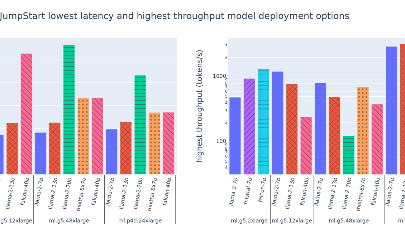
The following figure shows the lowest latencies (left) and highest throughput (right) values for deployment configurations across a variety of model types and instance types. Importantly, each of these model deployments use default configurations as provided by SageMaker JumpStart given the desired model ID and instance type for deployment.
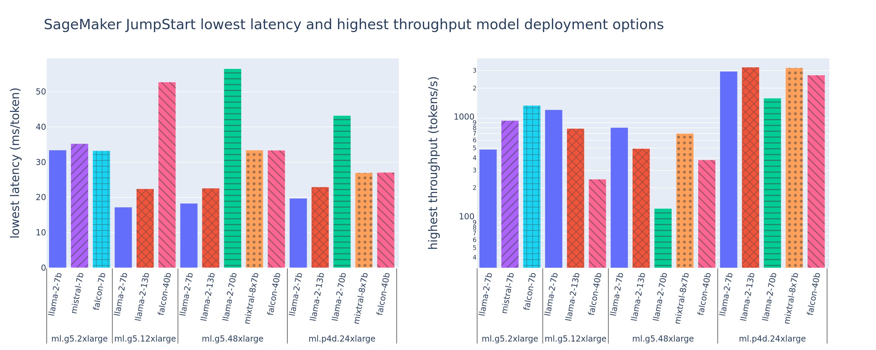
These latency and throughput values correspond to payloads with 256 input tokens and 256 output tokens. The lowest latency configuration limits model serving to a single concurrent request, and the highest throughput configuration maximizes the possible number of concurrent requests. As we can see in our benchmarking, increasing concurrent requests monotonically increases throughput with diminishing improvement for large concurrent requests. Additionally, models are fully sharded on the supported instance. For example, because the ml.g5.48xlarge instance has 8 GPUs, all SageMaker JumpStart models using this instance are sharded using tensor parallelism on all eight available accelerators.
We can note a few takeaways from this figure. First, not all models are supported on all instances; some smaller models, such as Falcon 7B, don’t support model sharding, whereas larger models have higher compute resource requirements. Second, as sharding increases, performance typically improves, but may not necessarily improve for small models. This is because small models such as 7B and 13B incur a substantial communication overhead when sharded across too many accelerators. We discuss this in more depth later. Finally, ml.p4d.24xlarge instances tend to have significantly better throughput due to memory bandwidth improvements of A100 over A10G GPUs. As we discuss later, the decision to use a particular instance type depends on your deployment requirements, including latency, throughput, and cost constraints.
How can you obtain these lowest latency and highest throughput configuration values? Let’s start by plotting latency vs. throughput for a Llama 2 7B endpoint on an ml.g5.12xlarge instance for a payload with 256 input tokens and 256 output tokens, as seen in the following curve. A similar curve exists for every deployed LLM endpoint.
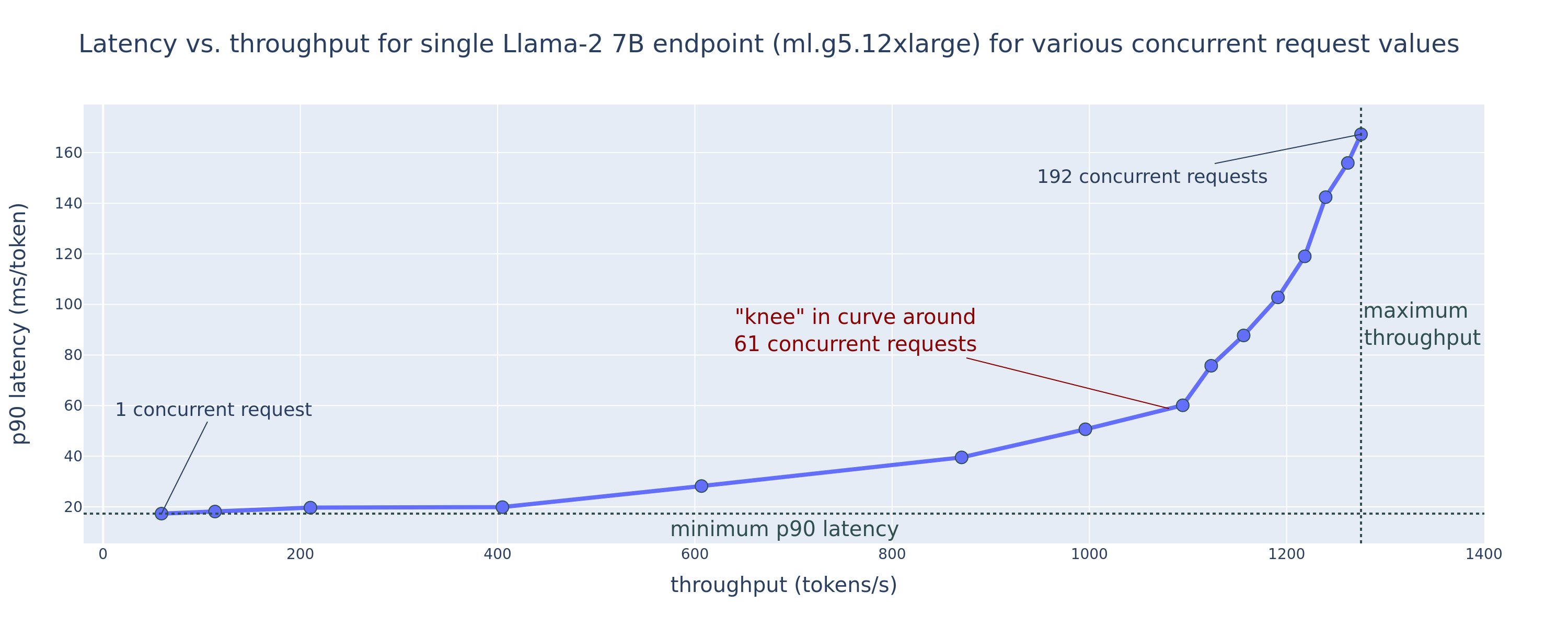
As concurrency increases, throughput and latency also monotonically increase. Therefore, the lowest latency point occurs at a concurrent request value of 1, and you can cost-effectively increase system throughput by increasing concurrent requests. There exists a distinct “knee” in this curve, where it’s obvious that the throughput gains associated with additional concurrency don’t outweigh the associated increase in latency. The exact location of this knee is use case-specific; some practitioners may define the knee at the point where a pre-specified latency requirement is exceeded (for example, 100 ms/token), whereas others may use load test benchmarks and queueing theory methods like the half-latency rule, and others may use theoretical accelerator specifications.
We also note that the maximum number of concurrent requests is limited. In the preceding figure, the line trace ends with 192 concurrent requests. The source of this limitation is the SageMaker invocation timeout limit, where SageMaker endpoints timeout an invocation response after 60 seconds. This setting is account-specific and not configurable for an individual endpoint. For LLMs, generating a large number of output tokens can take seconds or even minutes. Therefore, large input or output payloads can cause the invocation requests to fail. Furthermore, if the number of concurrent requests is very large, then many requests will experience large queue times, driving this 60-second timeout limit. For the purpose of this study, we use the timeout limit to define the maximum throughput possible for a model deployment. Importantly, although a SageMaker endpoint may handle a large number of concurrent requests without observing an invocation response timeout, you may want to define maximum concurrent requests with respect to the knee in the latency-throughput curve. This is likely the point at which you start to consider horizontal scaling, where a single endpoint provisions multiple instances with model replicas and load balances incoming requests between the replicas, to support more concurrent requests.
Taking this one step further, the following table contains benchmarking results for different configurations for the Llama 2 7B model, including different number of input and output tokens, instance types, and number of concurrent requests. Note that the preceding figure only plots a single row of this table.
| . |
Throughput (tokens/sec) |
Latency (ms/token) |
| Concurrent Requests |
1 |
2 |
4 |
8 |
16 |
32 |
64 |
128 |
256 |
512 |
1 |
2 |
4 |
8 |
16 |
32 |
64 |
128 |
256 |
512 |
| Number of total tokens: 512, Number of output tokens: 256 |
| ml.g5.2xlarge |
30 |
54 |
115 |
208 |
343 |
475 |
486 |
— |
— |
— |
33 |
33 |
35 |
39 |
48 |
97 |
159 |
— |
— |
— |
| ml.g5.12xlarge |
59 |
117 |
223 |
406 |
616 |
866 |
1098 |
1214 |
— |
— |
17 |
17 |
18 |
20 |
27 |
38 |
60 |
112 |
— |
— |
| ml.g5.48xlarge |
56 |
108 |
202 |
366 |
522 |
660 |
707 |
804 |
— |
— |
18 |
18 |
19 |
22 |
32 |
50 |
101 |
171 |
— |
— |
| ml.p4d.24xlarge |
49 |
85 |
178 |
353 |
654 |
1079 |
1544 |
2312 |
2905 |
2944 |
21 |
23 |
22 |
23 |
26 |
31 |
44 |
58 |
92 |
165 |
| Number of total tokens: 4096, Number of output tokens: 256 |
| ml.g5.2xlarge |
20 |
36 |
48 |
49 |
— |
— |
— |
— |
— |
— |
48 |
57 |
104 |
170 |
— |
— |
— |
— |
— |
— |
| ml.g5.12xlarge |
33 |
58 |
90 |
123 |
142 |
— |
— |
— |
— |
— |
31 |
34 |
48 |
73 |
132 |
— |
— |
— |
— |
— |
| ml.g5.48xlarge |
31 |
48 |
66 |
82 |
— |
— |
— |
— |
— |
— |
31 |
43 |
68 |
120 |
— |
— |
— |
— |
— |
— |
| ml.p4d.24xlarge |
39 |
73 |
124 |
202 |
278 |
290 |
— |
— |
— |
— |
26 |
27 |
33 |
43 |
66 |
107 |
— |
— |
— |
— |
We observe some additional patterns in this data. When increasing context size, latency increases and throughput decreases. For instance, on ml.g5.2xlarge with a concurrency of 1, throughput is 30 tokens/sec when the number of total tokens is 512, vs. 20 tokens/sec if the number of total tokens is 4,096. This is because it takes more time to process the larger input. We can also see that increasing GPU capability and sharding impacts the maximum throughput and maximum supported concurrent requests. The table shows that Llama 2 7B has notably different maximum throughput values for different instance types, and these maximum throughput values occur at different values of concurrent requests. These characteristics would drive an ML practitioner to justify the cost of one instance over another. For example, given a low latency requirement, the practitioner might select an ml.g5.12xlarge instance (4 A10G GPUs) over an ml.g5.2xlarge instance (1 A10G GPU). If given a high throughput requirement, the use of an ml.p4d.24xlarge instance (8 A100 GPUs) with full sharding would only be justified under high concurrency. Note, however, that it’s often beneficial to instead load multiple inference components of a 7B model on a single ml.p4d.24xlarge instance; such multi-model support is discussed later in this post.
The preceding observations were made for the Llama 2 7B model. However, similar patterns remain true for other models as well. A primary takeaway is that latency and throughput performance numbers are dependent on payload, instance type, and number of concurrent requests, so you will need to find the ideal configuration for your specific application. To generate the preceding numbers for your use case, you can run the linked notebook, where you can configure this load test analysis for your model, instance type, and payload.
Making sense of accelerator specifications
Selecting suitable hardware for LLM inference relies heavily on specific use cases, user experience goals, and the chosen LLM. This section attempts to create an understanding of the knee in the latency-throughput curve with respect to high-level principles based on accelerator specifications. These principles alone don’t suffice to make a decision: real benchmarks are necessary. The term device is used here to encompass all ML hardware accelerators. We assert the knee in the latency-throughput curve is driven by one of two factors:
- The accelerator has exhausted memory to cache KV matrices, so subsequent requests are queued
- The accelerator still has spare memory for the KV cache, but is using a large enough batch size that processing time is driven by compute operation latency rather than memory bandwidth
We typically prefer to be limited by the second factor because this implies the accelerator resources are saturated. Basically, you are maximizing the resources you payed for. Let’s explore this assertion in greater detail.
KV caching and device memory
Standard transformer attention mechanisms compute attention for each new token against all previous tokens. Most modern ML servers cache attention keys and values in device memory (DRAM) to avoid re-computation at every step. This is called this the KV cache, and it grows with batch size and sequence length. It defines how many user requests can be served in parallel and will determine the knee in the latency-throughput curve if the compute-bound regime in the second scenario mentioned earlier is not yet met, given the available DRAM. The following formula is a rough approximation for the maximum KV cache size.

In this formula, B is batch size and N is number of accelerators. For example, the Llama 2 7B model in FP16 (2 bytes/parameter) served on an A10G GPU (24 GB DRAM) consumes approximately 14 GB, leaving 10 GB for the KV cache. Plugging in the model’s full context length (N = 4096) and remaining parameters (n_layers=32, n_kv_attention_heads=32, and d_attention_head=128), this expression shows we are limited to serving a batch size of four users in parallel due to DRAM constraints. If you observe the corresponding benchmarks in the previous table, this is a good approximation for the observed knee in this latency-throughput curve. Methods such as grouped query attention (GQA) can reduce the KV cache size, in GQA’s case by the same factor it reduces the number of KV heads.
Arithmetic intensity and device memory bandwidth
The growth in the computational power of ML accelerators has outpaced their memory bandwidth, meaning they can perform many more computations on each byte of data in the amount of time it takes to access that byte.
The arithmetic intensity, or the ratio of compute operations to memory accesses, for an operation determines if it is limited by memory bandwidth or compute capacity on the selected hardware. For example, an A10G GPU (g5 instance type family) with 70 TFLOPS FP16 and 600 GB/sec bandwidth can compute approximately 116 ops/byte. An A100 GPU (p4d instance type family) can compute approximately 208 ops/byte. If the arithmetic intensity for a transformer model is under that value, it is memory-bound; if it is above, it is compute-bound. The attention mechanism for Llama 2 7B requires 62 ops/byte for batch size 1 (for an explanation, see A guide to LLM inference and performance), which means it is memory-bound. When the attention mechanism is memory-bound, expensive FLOPS are left unutilized.
There are two ways to better utilize the accelerator and increase arithmetic intensity: reduce the required memory accesses for the operation (this is what FlashAttention focuses on) or increase the batch size. However, we might not be able to increase our batch size enough to reach a compute-bound regime if our DRAM is too small to hold the corresponding KV cache. A crude approximation of the critical batch size B* that separates compute-bound from memory-bound regimes for standard GPT decoder inference is described by the following expression, where A_mb is the accelerator memory bandwidth, A_f is accelerator FLOPS, and N is the number of accelerators. This critical batch size can be derived by finding where memory access time equals computation time. Refer to this blog post to understand Equation 2 and its assumptions in greater detail.
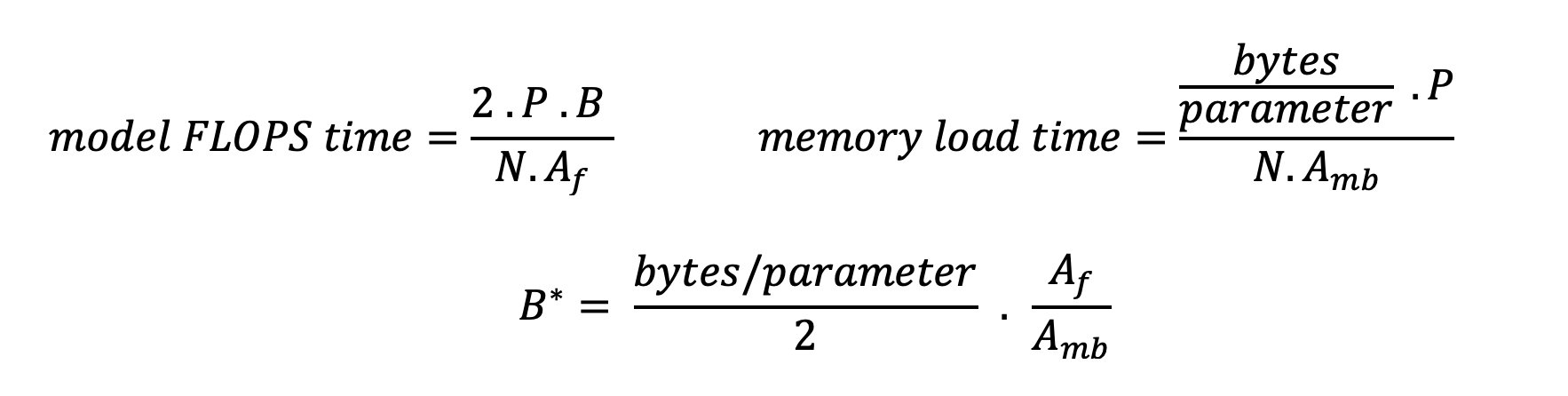
This is the same ops/byte ratio we previously calculated for A10G, so the critical batch size on this GPU is 116. One way to approach this theoretical, critical batch size is to increase model sharding and split the cache across more N accelerators. This effectively increases the KV cache capacity as well as the memory-bound batch size.
Another benefit of model sharding is splitting model parameter and data loading work across N accelerators. This type of sharding is a type of model parallelism also referred to as tensor parallelism. Naively, there is N times the memory bandwidth and compute power in aggregate. Assuming no overhead of any kind (communication, software, and so on), this would decrease decoding latency per token by N if we are memory-bound, because token decoding latency in this regime is bound by the time it takes to load the model weights and cache. In real life, however, increasing the degree of sharding results in increased communication between devices to share intermediate activations at every model layer. This communication speed is limited by the device interconnect bandwidth. It’s difficult to estimate its impact precisely (for details, see Model parallelism), but this can eventually stop yielding benefits or deteriorate performance — this is especially true for smaller models, because smaller data transfers lead to lower transfer rates.
To compare ML accelerators based on their specs, we recommend the following. First, calculate the approximate critical batch size for each accelerator type according to the second equation and the KV cache size for the critical batch size according to the first equation. You can then use the available DRAM on the accelerator to calculate the minimum number of accelerators required to fit the KV cache and model parameters. If deciding between multiple accelerators, prioritize accelerators in order of lowest cost per GB/sec of memory bandwidth. Finally, benchmark these configurations and verify what is the best cost/token for your upper bound of desired latency.
Select an endpoint deployment configuration
Many LLMs distributed by SageMaker JumpStart use the text-generation-inference (TGI) SageMaker container for model serving. The following table discusses how to adjust a variety of model serving parameters to either affect model serving which impacts the latency-throughput curve or protect the endpoint against requests that would overload the endpoint. These are the primary parameters you can use to configure your endpoint deployment for your use case. Unless otherwise specified, we use default text generation payload parameters and TGI environment variables.
| Environment Variable |
Description |
SageMaker JumpStart Default Value |
| Model serving configurations |
. |
. |
MAX_BATCH_PREFILL_TOKENS |
Limits the number of tokens in the prefill operation. This operation generates the KV cache for a new input prompt sequence. It is memory intensive and compute bound, so this value caps the number of tokens allowed in a single prefill operation. Decoding steps for other queries pause while prefill is occurring. |
4096 (TGI default) or model-specific maximum supported context length (SageMaker JumpStart provided), whichever is greater. |
MAX_BATCH_TOTAL_TOKENS |
Controls the maximum number of tokens to include within a batch during decoding, or a single forward pass through the model. Ideally, this is set to maximize the usage of all available hardware. |
Not specified (TGI default). TGI will set this value with respect to remaining CUDA memory during model warm up. |
SM_NUM_GPUS |
The number of shards to use. That is, the number of GPUs used to run the model using tensor parallelism. |
Instance dependent (SageMaker JumpStart provided). For each supported instance for a given model, SageMaker JumpStart provides the best setting for tensor parallelism. |
| Configurations to guard your endpoint (set these for your use case) |
. |
. |
MAX_TOTAL_TOKENS |
This caps the memory budget of a single client request by limiting the number of tokens in the input sequence plus the number of tokens in the output sequence (the max_new_tokens payload parameter). |
Model-specific maximum supported context length. For example, 4096 for Llama 2. |
MAX_INPUT_LENGTH |
Identifies the maximum allowed number of tokens in the input sequence for a single client request. Things to consider when increasing this value include: longer input sequences require more memory, which affects continuous batching, and many models have a supported context length that should not be exceeded. |
Model-specific maximum supported context length. For example, 4095 for Llama 2. |
MAX_CONCURRENT_REQUESTS |
The maximum number of concurrent requests allowed by the deployed endpoint. New requests beyond this limit will immediately raise a model overloaded error to prevent poor latency for the current processing requests. |
128 (TGI default). This setting allows you to obtain high throughput for a variety of use cases, but you should pin as appropriate to mitigate SageMaker invocation timeout errors. |
The TGI server uses continuous batching, which dynamically batches concurrent requests together to share a single model inference forward pass. There are two types of forward passes: prefill and decode. Each new request must run a single prefill forward pass to populate the KV cache for the input sequence tokens. After the KV cache is populated, a decode forward pass performs a single next-token prediction for all batched requests, which is iteratively repeated to produce the output sequence. As new requests are sent to the server, the next decode step must wait so the prefill step can run for the new requests. This must occur before those new requests are included in subsequent continuously batched decode steps. Due to hardware constraints, the continuous batching used for decoding may not include all requests. At this point, requests enter a processing queue and inference latency starts to significantly increase with only minor throughput gain.
It’s possible to separate LLM latency benchmarking analyses into prefill latency, decode latency, and queue latency. The time consumed by each of these components is fundamentally different in nature: prefill is a one-time computation, decoding occurs one time for each token in the output sequence, and queueing involves server batching processes. When multiple concurrent requests are being processed, it becomes difficult to disentangle the latencies from each of these components because the latency experienced by any given client request involves queue latencies driven by the need to prefill new concurrent requests as well as queue latencies driven by the inclusion of the request in batch decoding processes. For this reason, this post focuses on end-to-end processing latency. The knee in the latency-throughput curve occurs at the point of saturation where queue latencies start to significantly increase. This phenomenon occurs for any model inference server and is driven by accelerator specifications.
Common requirements during deployment include satisfying a minimum required throughput, maximum allowed latency, maximum cost per hour, and maximum cost to generate 1 million tokens. You should condition these requirements on payloads that represent end-user requests. A design to meet these requirements should consider many factors, including the specific model architecture, size of the model, instance types, and instance count (horizontal scaling). In the following sections, we focus on deploying endpoints to minimize latency, maximize throughput, and minimize cost. This analysis considers 512 total tokens and 256 output tokens.
Minimize latency
Latency is an important requirement in many real-time use cases. In the following table, we look at minimum latency for each model and each instance type. You can achieve minimum latency by setting MAX_CONCURRENT_REQUESTS = 1.
| Minimum Latency (ms/token) |
| Model ID |
ml.g5.2xlarge |
ml.g5.12xlarge |
ml.g5.48xlarge |
ml.p4d.24xlarge |
ml.p4de.24xlarge |
| Llama 2 7B |
33 |
17 |
18 |
20 |
— |
| Llama 2 7B Chat |
33 |
17 |
18 |
20 |
— |
| Llama 2 13B |
— |
22 |
23 |
23 |
— |
| Llama 2 13B Chat |
— |
23 |
23 |
23 |
— |
| Llama 2 70B |
— |
— |
57 |
43 |
— |
| Llama 2 70B Chat |
— |
— |
57 |
45 |
— |
| Mistral 7B |
35 |
— |
— |
— |
— |
| Mistral 7B Instruct |
35 |
— |
— |
— |
— |
| Mixtral 8x7B |
— |
— |
33 |
27 |
— |
| Falcon 7B |
33 |
— |
— |
— |
— |
| Falcon 7B Instruct |
33 |
— |
— |
— |
— |
| Falcon 40B |
— |
53 |
33 |
27 |
— |
| Falcon 40B Instruct |
— |
53 |
33 |
28 |
— |
| Falcon 180B |
— |
— |
— |
— |
42 |
| Falcon 180B Chat |
— |
— |
— |
— |
42 |
To achieve minimum latency for a model, you can use the following code while substituting your desired model ID and instance type:
from sagemaker.jumpstart.model import JumpStartModel

model = JumpStartModel(
    model_id="meta-textgeneration-llama-2-7b",
    model_version="3.*",
    instance_type="ml.g5.12xlarge",
    env={
        "MAX_CONCURRENT_REQUESTS": "1",
        "MAX_INPUT_TOKENS": "256",
        "MAX_TOTAL_TOKENS": "512",
    },
)
predictor = model.deploy(accept_eula=False)  # Change EULA acceptance to True
Note that the latency numbers change depending on the number of input and output tokens. However, the deployment process remains the same except the environment variables MAX_INPUT_TOKENS and MAX_TOTAL_TOKENS. Here, these environment variables are set to help guarantee endpoint latency requirements because larger input sequences may violate the latency requirement. Note that SageMaker JumpStart already provides the other optimal environment variables when selecting instance type; for instance, using ml.g5.12xlarge will set SM_NUM_GPUS to 4 in the model environment.
Maximize throughput
In this section, we maximize the number of generated tokens per second. This is typically achieved at the maximum valid concurrent requests for the model and the instance type. In the following table, we report the throughput achieved at the largest concurrent request value achieved before encountering a SageMaker invocation timeout for any request.
| Maximum Throughput (tokens/sec), Concurrent Requests |
| Model ID |
ml.g5.2xlarge |
ml.g5.12xlarge |
ml.g5.48xlarge |
ml.p4d.24xlarge |
ml.p4de.24xlarge |
| Llama 2 7B |
486 (64) |
1214 (128) |
804 (128) |
2945 (512) |
— |
| Llama 2 7B Chat |
493 (64) |
1207 (128) |
932 (128) |
3012 (512) |
— |
| Llama 2 13B |
— |
787 (128) |
496 (64) |
3245 (512) |
— |
| Llama 2 13B Chat |
— |
782 (128) |
505 (64) |
3310 (512) |
— |
| Llama 2 70B |
— |
— |
124 (16) |
1585 (256) |
— |
| Llama 2 70B Chat |
— |
— |
114 (16) |
1546 (256) |
— |
| Mistral 7B |
947 (64) |
— |
— |
— |
— |
| Mistral 7B Instruct |
986 (128) |
— |
— |
— |
— |
| Mixtral 8x7B |
— |
— |
701 (128) |
3196 (512) |
— |
| Falcon 7B |
1340 (128) |
— |
— |
— |
— |
| Falcon 7B Instruct |
1313 (128) |
— |
— |
— |
— |
| Falcon 40B |
— |
244 (32) |
382 (64) |
2699 (512) |
— |
| Falcon 40B Instruct |
— |
245 (32) |
415 (64) |
2675 (512) |
— |
| Falcon 180B |
— |
— |
— |
— |
1100 (128) |
| Falcon 180B Chat |
— |
— |
— |
— |
1081 (128) |
To achieve maximum throughput for a model, you can use the following code:
from sagemaker.jumpstart.model import JumpStartModel

model = JumpStartModel(
    model_id="meta-textgeneration-llama-2-7b",
    model_version="3.*",
    instance_type="ml.g5.12xlarge",
    env={
        "MAX_CONCURRENT_REQUESTS": "128",  # For your application, identify it from the benchmarking table with the maximum feasible concurrent requests.
        "MAX_INPUT_TOKENS": "256",
        "MAX_TOTAL_TOKENS": "512",
    },
)
predictor = model.deploy(accept_eula=False)  # Change EULA acceptance to True
Note that the maximum number of concurrent requests depends on the model type, instance type, maximum number of input tokens, and maximum number of output tokens. Therefore, you should set these parameters before setting MAX_CONCURRENT_REQUESTS.
Also note that a user interested in minimizing latency is often at odds with a user interested in maximizing throughput. The former is interested in real-time responses, whereas the latter is interested in batch processing such that the endpoint queue is always saturated, thereby minimizing processing downtime. Users who want to maximize throughput conditioned on latency requirements are often interested in operating at the knee in the latency-throughput curve.
Minimize cost
The first option to minimize cost involves minimizing cost per hour. With this, you can deploy a selected model on the SageMaker instance with the lowest cost per hour. For real-time pricing of SageMaker instances, refer to Amazon SageMaker pricing. In general, the default instance type for SageMaker JumpStart LLMs is the lowest-cost deployment option.
The second option to minimize cost involves minimizing the cost to generate 1 million tokens. This is a simple transformation of the table we discussed earlier to maximize throughput, where you can first compute the time it takes in hours to generate 1 million tokens (1e6 / throughput / 3600). You can then multiply this time to generate 1 million tokens with the price per hour of the specified SageMaker instance.
Note that instances with the lowest cost per hour aren’t the same as instances with the lowest cost to generate 1 million tokens. For instance, if the invocation requests are sporadic, an instance with the lowest cost per hour might be optimal, whereas in the throttling scenarios, the lowest cost to generate a million tokens might be more appropriate.
Tensor parallel vs. multi-model trade-off
In all previous analyses, we considered deploying a single model replica with a tensor parallel degree equal to the number of GPUs on the deployment instance type. This is the default SageMaker JumpStart behavior. However, as previously noted, sharding a model can improve model latency and throughput only up to a certain limit, beyond which inter-device communication requirements dominate computation time. This implies that it’s often beneficial to deploy multiple models with a lower tensor parallel degree on a single instance rather than a single model with a higher tensor parallel degree.
Here, we deploy Llama 2 7B and 13B endpoints on ml.p4d.24xlarge instances with tensor parallel (TP) degrees of 1, 2, 4, and 8. For clarity in model behavior, each of these endpoints only load a single model.
| . |
Throughput (tokens/sec) |
Latency (ms/token) |
| Concurrent Requests |
1 |
2 |
4 |
8 |
16 |
32 |
64 |
128 |
256 |
512 |
1 |
2 |
4 |
8 |
16 |
32 |
64 |
128 |
256 |
512 |
| TP Degree |
Llama 2 13B |
| 1 |
38 |
74 |
147 |
278 |
443 |
612 |
683 |
722 |
— |
— |
26 |
27 |
27 |
29 |
37 |
45 |
87 |
174 |
— |
— |
| 2 |
49 |
92 |
183 |
351 |
604 |
985 |
1435 |
1686 |
1726 |
— |
21 |
22 |
22 |
22 |
25 |
32 |
46 |
91 |
159 |
— |
| 4 |
46 |
94 |
181 |
343 |
655 |
1073 |
1796 |
2408 |
2764 |
2819 |
23 |
21 |
21 |
24 |
25 |
30 |
37 |
57 |
111 |
172 |
| 8 |
44 |
86 |
158 |
311 |
552 |
1015 |
1654 |
2450 |
3087 |
3180 |
22 |
24 |
26 |
26 |
29 |
36 |
42 |
57 |
95 |
152 |
| . |
Llama 2 7B |
| 1 |
62 |
121 |
237 |
439 |
778 |
1122 |
1569 |
1773 |
1775 |
— |
16 |
16 |
17 |
18 |
22 |
28 |
43 |
88 |
151 |
— |
| 2 |
62 |
122 |
239 |
458 |
780 |
1328 |
1773 |
2440 |
2730 |
2811 |
16 |
16 |
17 |
18 |
21 |
25 |
38 |
56 |
103 |
182 |
| 4 |
60 |
106 |
211 |
420 |
781 |
1230 |
2206 |
3040 |
3489 |
3752 |
17 |
19 |
20 |
18 |
22 |
27 |
31 |
45 |
82 |
132 |
| 8 |
49 |
97 |
179 |
333 |
612 |
1081 |
1652 |
2292 |
2963 |
3004 |
22 |
20 |
24 |
26 |
27 |
33 |
41 |
65 |
108 |
167 |
Our previous analyses already showed significant throughput advantages on ml.p4d.24xlarge instances, which often translates to better performance in terms of cost to generate 1 million tokens over the g5 instance family under high concurrent request load conditions. This analysis clearly demonstrates that you should consider the trade-off between model sharding and model replication within a single instance; that is, a fully sharded model is not typically the best use of ml.p4d.24xlarge compute resources for 7B and 13B model families. In fact, for the 7B model family, you obtain the best throughput for a single model replica with a tensor parallel degree of 4 instead of 8.
From here, you can extrapolate that the highest throughput configuration for the 7B model involves a tensor parallel degree of 1 with eight model replicas, and the highest throughput configuration for the 13B model is likely a tensor parallel degree of 2 with four model replicas. To learn more about how to accomplish this, refer to Reduce model deployment costs by 50% on average using the latest features of Amazon SageMaker, which demonstrates the use of inference component-based endpoints. Due to load balancing techniques, server routing, and sharing of CPU resources, you might not fully achieve throughput improvements exactly equal to the number of replicas times the throughput for a single replica.
Horizontal scaling
As observed earlier, each endpoint deployment has a limitation on the number of concurrent requests depending on the number of input and output tokens as well as the instance type. If this doesn’t meet your throughput or concurrent request requirement, you can scale up to utilize more than one instance behind the deployed endpoint. SageMaker automatically performs load balancing of queries between instances. For example, the following code deploys an endpoint supported by three instances:
model = JumpStartModel(
    model_id="meta-textgeneration-llama-2-7b",
    model_version="3.*",
    instance_type="ml.g5.2xlarge",
)
predictor = model.deploy(
    accept_eula=False,  # Change EULA acceptance to True
    initial_instance_count = 3,
)
The following table shows the throughput gain as a factor of number of instances for the Llama 2 7B model.
| . |
. |
Throughput (tokens/sec) |
Latency (ms/token) |
| . |
Concurrent Requests |
1 |
2 |
4 |
8 |
16 |
32 |
64 |
128 |
1 |
2 |
4 |
8 |
16 |
32 |
64 |
128 |
| Instance Count |
Instance Type |
Number of total tokens: 512, Number of output tokens: 256 |
| 1 |
ml.g5.2xlarge |
30 |
60 |
115 |
210 |
351 |
484 |
492 |
— |
32 |
33 |
34 |
37 |
45 |
93 |
160 |
— |
| 2 |
ml.g5.2xlarge |
30 |
60 |
115 |
221 |
400 |
642 |
922 |
949 |
32 |
33 |
34 |
37 |
42 |
53 |
94 |
167 |
| 3 |
ml.g5.2xlarge |
30 |
60 |
118 |
228 |
421 |
731 |
1170 |
1400 |
32 |
33 |
34 |
36 |
39 |
47 |
57 |
110 |
Notably, the knee in the latency-throughput curve shifts to the right because higher instance counts can handle larger numbers of concurrent requests within the multi-instance endpoint. For this table, the concurrent request value is for the entire endpoint, not the number of concurrent requests that each individual instance receives.
You can also use autoscaling, a feature to monitor your workloads and dynamically adjust the capacity to maintain steady and predictable performance at the possible lowest cost. This is beyond the scope of this post. To learn more about autoscaling, refer to Configuring autoscaling inference endpoints in Amazon SageMaker.
Invoke endpoint with concurrent requests
Let’s suppose you have a large batch of queries that you would like to use to generate responses from a deployed model under high throughput conditions. For example, in the following code block, we compile a list of 1,000 payloads, with each payload requesting the generation of 100 tokens. In all, we are requesting the generation of 100,000 tokens.
payload = {
    "inputs": "I believe the meaning of life is to ",
    "parameters": {"max_new_tokens": 100, "details": True},
}
total_requests = 1000
payloads = [payload,] * total_requests
When sending a large number of requests to the SageMaker runtime API, you may experience throttling errors. To mitigate this, you can create a custom SageMaker runtime client that increases the number of retry attempts. You can provide the resulting SageMaker session object to either the JumpStartModel constructor or sagemaker.predictor.retrieve_default if you would like to attach a new predictor to an already deployed endpoint. In the following code, we use this session object when deploying a Llama 2 model with default SageMaker JumpStart configurations:
import boto3
from botocore.config import Config
from sagemaker.session import Session
from sagemaker.jumpstart.model import JumpStartModel

sagemaker_session = Session(
    sagemaker_runtime_client=boto3.client(
        "sagemaker-runtime",
        config=Config(connect_timeout=10, retries={"mode": "standard", "total_max_attempts": 20}),
    )
)
model = JumpStartModel(
    model_id="meta-textgeneration-llama-2-7b",
    model_version="3.*",
    sagemaker_session=sagemaker_session
)
predictor = model.deploy(accept_eula=False)  # Change EULA acceptance to True
This deployed endpoint has MAX_CONCURRENT_REQUESTS = 128 by default. In the following block, we use the concurrent futures library to iterate over invoking the endpoint for all payloads with 128 worker threads. At most, the endpoint will process 128 concurrent requests, and whenever a request returns a response, the executor will immediately send a new request to the endpoint.
import time
from concurrent import futures

concurrent_requests = 128

time_start = time.time()
with futures.ThreadPoolExecutor(max_workers=concurrent_requests) as executor:
    responses = list(executor.map(predictor.predict, payloads))

total_tokens = sum([response[0]["details"]["generated_tokens"] for response in responses])
token_throughput = total_tokens / (time.time() - time_start)
This results in generating 100,000 total tokens with a throughput of 1255 tokens/sec on a single ml.g5.2xlarge instance. This takes approximately 80 seconds to process.
Note that this throughput value is notably different than the maximum throughput for Llama 2 7B on ml.g5.2xlarge in the previous tables of this post (486 tokens/sec at 64 concurrent requests). This is because the input payload uses 8 tokens instead of 256, the output token count is 100 instead of 256, and the smaller token counts allow for 128 concurrent requests. This is a final reminder that all latency and throughput numbers are payload dependent! Changing payload token counts will affect batching processes during model serving, which will in turn affect the emergent prefill, decode, and queue times for your application.
Conclusion
In this post, we presented benchmarking of SageMaker JumpStart LLMs, including Llama 2, Mistral, and Falcon. We also presented a guide to optimize latency, throughput, and cost for your endpoint deployment configuration. You can get started by running the associated notebook to benchmark your use case.
About the Authors
 Dr. Kyle Ulrich is an Applied Scientist with the Amazon SageMaker JumpStart team. His research interests include scalable machine learning algorithms, computer vision, time series, Bayesian non-parametrics, and Gaussian processes. His PhD is from Duke University and he has published papers in NeurIPS, Cell, and Neuron.
 Dr. Vivek Madan is an Applied Scientist with the Amazon SageMaker JumpStart team. He got his PhD from University of Illinois at Urbana-Champaign and was a Post Doctoral Researcher at Georgia Tech. He is an active researcher in machine learning and algorithm design and has published papers in EMNLP, ICLR, COLT, FOCS, and SODA conferences.
 Dr. Ashish Khetan is a Senior Applied Scientist with Amazon SageMaker JumpStart and helps develop machine learning algorithms. He got his PhD from University of Illinois Urbana-Champaign. He is an active researcher in machine learning and statistical inference, and has published many papers in NeurIPS, ICML, ICLR, JMLR, ACL, and EMNLP conferences.
 João Moura is a Senior AI/ML Specialist Solutions Architect at AWS. João helps AWS customers – from small startups to large enterprises – train and deploy large models efficiently, and more broadly build ML platforms on AWS.
Read More


 We’re publishing an AI Opportunity whitepaper to help ASEAN governments tap into AI’s vast potential.