Two salient limitations have long hindered the relevance of optimal transport methods to machine learning. First, the computational cost of standard sample-based solvers (when used on batches of samples) is prohibitive. Second, the mass conservation constraint makes OT solvers too rigid in practice: because they must match textit{all} points from both measures, their output can be heavily influenced by outliers. A flurry of recent works has addressed these computational and modeling limitations. Still it has resulted in two separate strains of methods: While the computational outlook was…Apple Machine Learning Research
FastSR-NeRF: Improving NeRF Efficiency on Consumer Devices with A Simple Super-Resolution Pipeline
Super-resolution (SR) techniques have recently been proposed to upscale the outputs of neural radiance fields (NeRF) and generate high-quality images with enhanced inference speeds. However, existing NeRF+SR methods increase training overhead by using extra input features, loss functions, and/or expensive training procedures such as knowledge distillation. In this paper, we aim to leverage SR for efficiency gains without costly training or architectural changes. Specifically, we build a simple NeRF+SR pipeline that directly combines existing modules, and we propose a lightweight augmentation…Apple Machine Learning Research
Simulation-based Inference for Cardiovascular Models
This paper was accepted at the workshop Machine Learning and the Physical Sciences at NeurIPS 2023.
Over the past decades, hemodynamics simulators have steadily evolved and have become tools of choice for studying cardiovascular systems in-silico. This comes naturally at the cost of increasing complexity since state-of-the-art models are non-linear partial differential equations depending on many parameters. While such tools are routinely used to simulate hemodynamics given physiological parameters, solving the related inverse problems — mapping waveforms to physiological parameters — has…Apple Machine Learning Research
Bin Prediction for Better Conformal Prediction
This paper was accepted at the workshop on Regulatable ML at NeurIPS 2023.
Conformal Prediction (CP) is a method of estimating risk or uncertainty when using Machine Learning to help abide by common Risk Management regulations often seen in fields like healthcare and finance. CP for regression can be challenging, especially when the output distribution is heteroscedastic, multimodal, or skewed. Some of the issues can be addressed by estimating a distribution over the output, but in reality, such approaches can be sensitive to estimation error and yield unstable intervals. Here, we circumvent…Apple Machine Learning Research
One Wide Feedforward is All You Need
This paper was accepted at WMT conference at EMNLP.
The Transformer architecture has two main non-embedding components: Attention and the Feed Forward Network (FFN). Attention captures interdependencies between words regardless of their position, while the FFN non-linearly transforms each input token independently. In this work, we explore the role of FFN and find that despite, and find that despite taking up a significant fraction of the model’s parameters, it is highly redundant. Concretely, we are able to substantially reduce the number of parameters with only a modest drop in accuracy by…Apple Machine Learning Research
Hybrid Model Learning for Cardiovascular Biomarkers Inference
This paper was accepted at the workshop Deep Generative Models for Health at NeurIPS 2023.
Cardiovascular diseases (CVDs) are a major global health concern, making the longitudinal monitoring of cardiovascular biomarkers vital for early diagnosis and intervention. A core challenge is the inference of cardiac pulse parameters from pulse waves, especially when acquired from wearable sensors at peripheral body locations. Traditional machine learning (ML) approaches face hurdles in this context due to the scarcity of labeled data, primarily sourced from clinical settings. Simultaneously, physical…Apple Machine Learning Research
Vision-language models that can handle multi-image inputs
Attention-based representation of multi-image inputs improves performance on downstream vision-language tasks.Read More
Reduce inference time for BERT models using neural architecture search and SageMaker Automated Model Tuning
In this post, we demonstrate how to use neural architecture search (NAS) based structural pruning to compress a fine-tuned BERT model to improve model performance and reduce inference times. Pre-trained language models (PLMs) are undergoing rapid commercial and enterprise adoption in the areas of productivity tools, customer service, search and recommendations, business process automation, and content creation. Deploying PLM inference endpoints is typically associated with higher latency and higher infrastructure costs due to the compute requirements and reduced computational efficiency due to the large number of parameters. Pruning a PLM reduces the size and complexity of the model while retaining its predictive capabilities. Pruned PLMs achieve a smaller memory footprint and lower latency. We demonstrate that by pruning a PLM and trading off parameter count and validation error for a specific target task, and are able to achieve faster response times when compared to the base PLM model.
Multi-objective optimization is an area of decision-making that optimizes more than one objective function, such as memory consumption, training time, and compute resources, to be optimized simultaneously. Structural pruning is a technique to reduce the size and computational requirements of PLM by pruning layers or neurons/nodes while attempting to preserve model accuracy. By removing layers, structural pruning achieves higher compression rates, which leads to hardware-friendly structured sparsity that reduces runtimes and response times. Applying a structural pruning technique to a PLM model results in a lighter-weight model with a lower memory footprint that, when hosted as an inference endpoint in SageMaker, offers improved resource efficiency and reduced cost when compared to the original fine-tuned PLM.
The concepts illustrated in this post can be applied to applications that use PLM features, such as recommendation systems, sentiment analysis, and search engines. Specifically, you can use this approach if you have dedicated machine learning (ML) and data science teams who fine-tune their own PLM models using domain-specific datasets and deploy a large number of inference endpoints using Amazon SageMaker. One example is an online retailer who deploys a large number of inference endpoints for text summarization, product catalog classification, and product feedback sentiment classification. Another example might be a healthcare provider who uses PLM inference endpoints for clinical document classification, named entity recognition from medical reports, medical chatbots, and patient risk stratification.
Solution overview
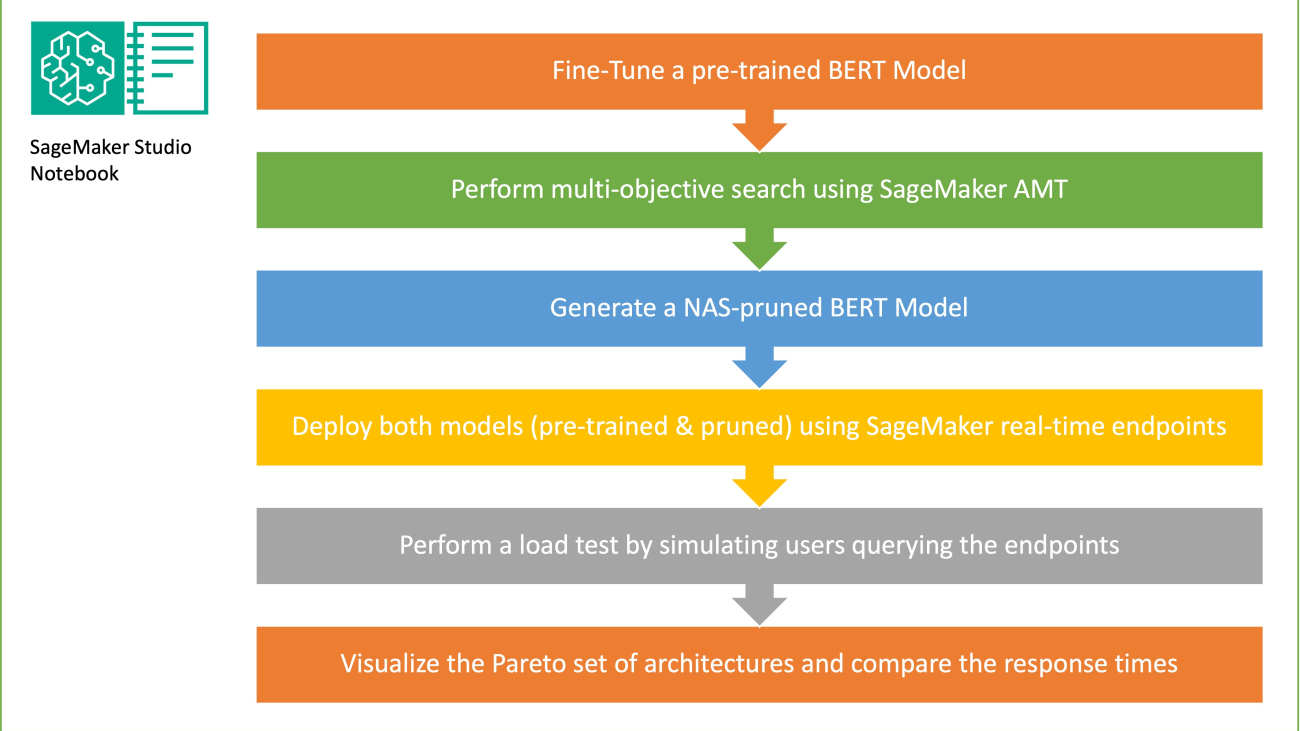
In this section, we present the overall workflow and explain the approach. First, we use an Amazon SageMaker Studio notebook to fine-tune a pre-trained BERT model on a target task using a domain-specific dataset. BERT (Bidirectional Encoder Representations from Transformers) is a pre-trained language model based on the transformer architecture used for natural language processing (NLP) tasks. Neural architecture search (NAS) is an approach for automating the design of artificial neural networks and is closely related to hyperparameter optimization, a widely used approach in the field of machine learning. The goal of NAS is to find the optimal architecture for a given problem by searching over a large set of candidate architectures using techniques such as gradient-free optimization or by optimizing the desired metrics. The performance of the architecture is typically measured using metrics such as validation loss. SageMaker Automatic Model Tuning (AMT) automates the tedious and complex process of finding the optimal combinations of hyperparameters of the ML model that yield the best model performance. AMT uses intelligent search algorithms and iterative evaluations using a range of hyperparameters that you specify. It chooses the hyperparameter values that creates a model that performs the best, as measured by performance metrics such as accuracy and F-1 score.
The fine-tuning approach described in this post is generic and can be applied to any text-based dataset. The task assigned to the BERT PLM can be a text-based task such as sentiment analysis, text classification, or Q&A. In this demo, the target task is a binary classification problem where BERT is used to identify, from a dataset that consists of a collection of pairs of text fragments, whether the meaning of one text fragment can be inferred from the other fragment. We use the Recognizing Textual Entailment dataset from the GLUE benchmarking suite. We perform a multi-objective search using SageMaker AMT to identify the sub-networks that offer optimal trade-offs between parameter count and prediction accuracy for the target task. When performing a multi-objective search, we start with defining the accuracy and parameter count as the objectives that we are aiming to optimize.
Within the BERT PLM network, there can be modular, self-contained sub-networks that allow the model to have specialized capabilities such as language understanding and knowledge representation. BERT PLM uses a multi-headed self-attention sub-network and a feed-forward sub-network. A multi-headed, self-attention layer allows BERT to relate different positions of a single sequence in order to compute a representation of the sequence by allowing multiple heads to attend to multiple context signals. The input is split into multiple subspaces and self-attention is applied to each of the subspaces separately. Multiple heads in a transformer PLM allow the model to jointly attend to information from different representation subspaces. A feed-forward sub-network is a simple neural network that takes the output from the multi-headed self-attention sub-network, processes the data, and returns the final encoder representations.
The goal of random sub-network sampling is to train smaller BERT models that can perform well enough on target tasks. We sample 100 random sub-networks from the fine-tuned base BERT model and evaluate 10 networks simultaneously. The trained sub-networks are evaluated for the objective metrics and the final model is chosen based on the trade-offs found between the objective metrics. We visualize the Pareto front for the sampled sub-networks, which contains the pruned model that offers the optimal trade-off between model accuracy and model size. We select the candidate sub-network (NAS-pruned BERT model) based on the model size and model accuracy that we are willing to trade off. Next, we host the endpoints, the pre-trained BERT base model, and the NAS-pruned BERT model using SageMaker. To perform load testing, we use Locust, an open source load testing tool that you can implement using Python. We run load testing on both endpoints using Locust and visualize the results using the Pareto front to illustrate the trade-off between response times and accuracy for both models. The following diagram provides an overview of the workflow explained in this post.

Prerequisites
For this post, the following prerequisites are required:
- An AWS account with access to the AWS Management Console
- A SageMaker domain, SageMaker user profile, and SageMaker Studio
- An IAM execution role for the SageMaker Studio Domain user
You also need to increase the service quota to access at least three instances of ml.g4dn.xlarge instances in SageMaker. The instance type ml.g4dn.xlarge is the cost efficient GPU instance that allows you to run PyTorch natively. To increase the service quota, complete the following steps:
- On the console, navigate to Service Quotas.
- For Manage quotas, choose Amazon SageMaker, then choose View quotas.

- Search for “ml-g4dn.xlarge for training job usage” and select the quota item.
- Choose Request increase at account-level.

- For Increase quota value, enter a value of 5 or higher.
- Choose Request.
The requested quota approval may take some time to complete depending on the account permissions.

- Open SageMaker Studio from the SageMaker console.

- Choose System terminal under Utilities and files.

- Run the following command to clone the GitHub repo to the SageMaker Studio instance:
- Navigate to
amazon-sagemaker-examples/hyperparameter_tuning/neural_architecture_search_llm. - Open the file
nas_for_llm_with_amt.ipynb. - Set up the environment with an
ml.g4dn.xlargeinstance and choose Select.

Set up the pre-trained BERT model
In this section, we import the Recognizing Textual Entailment dataset from the dataset library and split the dataset into training and validation sets. This dataset consists of pairs of sentences. The task of the BERT PLM is to recognize, given two text fragments, whether the meaning of one text fragment can be inferred from the other fragment. In the following example, we can infer the meaning of the first phrase from the second phrase:
We load the textual recognizing entailment dataset from the GLUE benchmarking suite via the dataset library from Hugging Face within our training script (./training.py). We split the original training dataset from GLUE into a training and validation set. In our approach, we fine-tune the base BERT model using the training dataset, then we perform a multi-objective search to identify the set of sub-networks that optimally balance between the objective metrics. We use the training dataset exclusively for fine-tuning the BERT model. However, we use validation data for the multi-objective search by measuring accuracy on the holdout validation dataset.
Fine-tune the BERT PLM using a domain-specific dataset
The typical use cases for a raw BERT model include next sentence prediction or masked language modeling. To use the base BERT model for downstream tasks such as textual recognizing entailment, we have to further fine-tune the model using a domain-specific dataset. You can use a fine-tuned BERT model for tasks such as sequence classification, question answering, and token classification. However, for the purposes of this demo, we use the fine-tuned model for binary classification. We fine-tune the pre-trained BERT model with the training dataset that we prepared previously, using the following hyperparameters:
We save the checkpoint of the model training to an Amazon Simple Storage Service (Amazon S3) bucket, so that the model can be loaded during the NAS-based multi-objective search. Before we train the model, we define the metrics such as epoch, training loss, number of parameters, and validation error:
After the fine-tuning process starts, the training job takes around 15 minutes to complete.
Perform a multi-objective search to select sub-networks and visualize the results
In the next step, we perform a multi-objective search on the fine-tuned base BERT model by sampling random sub-networks using SageMaker AMT. To access a sub-network within the super-network (the fine-tuned BERT model), we mask out all the components of the PLM that are not part of the sub-network. Masking a super-network to find sub-networks in a PLM is a technique used to isolate and identify patterns of the model’s behavior. Note that Hugging Face transformers needs the hidden size to be a multiple of the number of heads. The hidden size in a transformer PLM controls the size of the hidden state vector space, which impacts the model’s ability to learn complex representations and patterns in the data. In a BERT PLM, the hidden state vector is of a fixed size (768). We can’t change the hidden size, and therefore the number of heads has to be in [1, 3, 6, 12].
In contrast to single-objective optimization, in the multi-objective setting, we typically don’t have a single solution that simultaneously optimizes all objectives. Instead, we aim to collect a set of solutions that dominate all other solutions in at least one objective (such as validation error). Now we can start the multi-objective search through AMT by setting the metrics that we want to reduce (validation error and number of parameters). The random sub-networks are defined by the parameter max_jobs and the number of simultaneous jobs is defined by the parameter max_parallel_jobs. The code to load the model checkpoint and evaluate the sub-network is available in the evaluate_subnetwork.py script.
The AMT tuning job takes approximately 2 hours and 20 minutes to run. After the AMT tuning job runs successfully, we parse the job’s history and collect the sub-network’s configurations, such as number of heads, number of layers, number of units, and the corresponding metrics such as validation error and number of parameters. The following screenshot shows the summary of a successful AMT tuner job.
Next, we visualize the results using a Pareto set (also known as Pareto frontier or Pareto optimal set), which helps us identify optimal sets of sub-networks that dominate all other sub-networks in the objective metric (validation error):
First, we collect the data from the AMT tuning job. Then then we plot the Pareto set using matplotlob.pyplot with number of parameters in the x axis and validation error in the y axis. This implies that when we move from one sub-network of the Pareto set to another, we must either sacrifice performance or model size but improve the other. Ultimately, the Pareto set provides us the flexibility to choose the sub-network that best suits our preferences. We can decide how much we want to reduce the size of our network and how much performance we are willing to sacrifice.

Deploy the fine-tuned BERT model and the NAS-optimized sub-network model using SageMaker
Next, we deploy the largest model in our Pareto set that leads to the smallest amount of performance degeneration to a SageMaker endpoint. The best model is the one that provides an optimal trade-off between the validation error and the number of parameters for our use case.
Model comparison
We took a pre-trained base BERT model, fine-tuned it using a domain-specific dataset, ran a NAS search to identify dominant sub-networks based on the objective metrics, and deployed the pruned model on a SageMaker endpoint. In addition, we took the pre-trained base BERT model and deployed the base model on a second SageMaker endpoint. Next, we ran load-testing using Locust on both inference endpoints and evaluated the performance in terms of response time.
First, we import the necessary Locust and Boto3 libraries. Then we construct a request metadata and record the start time to be used for load testing. Then the payload is passed to the SageMaker endpoint invoke API via the BotoClient to simulate real user requests. We use Locust to spawn multiple virtual users to send requests in parallel and measure the endpoint performance under the load. Tests are run by increasing the number of users for each of the two endpoints, respectively. After the tests are completed, Locust outputs a request statistics CSV file for each of the deployed models.
Next, we generate the response time plots from the CSV files downloaded after running the tests with Locust. The purpose of plotting the response time vs. the number of users is to analyze the load testing results by visualizing the impact of the response time of the model endpoints. In the following chart, we can see that the NAS-pruned model endpoint achieves a lower response time compared to the base BERT model endpoint.

In the second chart, which is an extension of the first chart, we observe that after around 70 users, SageMaker starts to throttle the base BERT model endpoint and throws an exception. However, for the NAS-pruned model endpoint, the throttling happens between 90–100 users and with a lower response time.

From the two charts, we observe that the pruned model has a faster response time and scales better when compared to the unpruned model. As we scale the number of inference endpoints, as is the case with users who deploy a large number of inference endpoints for their PLM applications, the cost benefits and performance improvement start to become quite substantial.
Clean up
To delete the SageMaker endpoints for the fine-tuned base BERT model and the NAS-pruned model, complete the following steps:
- On the SageMaker console, choose Inference and Endpoints in the navigation pane.
- Select the endpoint and delete it.
Alternatively, from the SageMaker Studio notebook, run the following commands by providing the endpoint names:
Conclusion
In this post, we discussed how to use NAS to prune a fine-tuned BERT model. We first trained a base BERT model using domain-specific data and deployed it to a SageMaker endpoint. We performed a multi-objective search on the fine-tuned base BERT model using SageMaker AMT for a target task. We visualized the Pareto front and selected the Pareto optimal NAS-pruned BERT model and deployed the model to a second SageMaker endpoint. We performed load testing using Locust to simulate users querying both the endpoints, and measured and recorded the response times in a CSV file. We plotted the response time vs. the number of users for both the models.
We observed that the pruned BERT model performed significantly better in both response time and instance throttling threshold. We concluded that the NAS-pruned model was more resilient to an increased load on the endpoint, maintaining a lower response time even as more users stressed the system compared to the base BERT model. You can apply the NAS technique described in this post to any large language model to find a pruned model that can perform the target task with significantly lower response time. You can further optimize the approach by using latency as a parameter in addition to validation loss.
Although we use NAS in this post, quantization is another common approach used to optimize and compress PLM models. Quantization reduces the precision of the weights and activations in a trained network from 32-bit floating point to lower bit widths such as 8-bit or 16-bit integers, which results in a compressed model that generates faster inference. Quantization doesn’t reduce the number of parameters; instead it reduces the precision of the existing parameters to get a compressed model. NAS pruning removes redundant networks in a PLM, which creates a sparse model with fewer parameters. Typically, NAS pruning and quantization are used together to compress large PLMs to maintain model accuracy, reduce validation losses while improving performance, and reduce model size. The other commonly used techniques to reduce the size of PLMs include knowledge distillation, matrix factorization, and distillation cascades.
The approach proposed in the blogpost is suitable for teams that use SageMaker to train and fine-tune the models using domain-specific data and deploy the endpoints to generate inference. If you’re looking for a fully managed service that offers a choice of high-performing foundation models needed to build generative AI applications, consider using Amazon Bedrock. If you’re looking for pre-trained, open source models for a wide range of business use cases and want to access solution templates and example notebooks, consider using Amazon SageMaker JumpStart. A pre-trained version of the Hugging Face BERT base cased model that we used in this post is also available from SageMaker JumpStart.
About the Authors
 Aparajithan Vaidyanathan is a Principal Enterprise Solutions Architect at AWS. He is a Cloud Architect with 24+ years of experience designing and developing enterprise, large-scale and distributed software systems. He specializes in Generative AI and Machine Learning Data Engineering. He is an aspiring marathon runner and his hobbies include hiking, bike riding and spending time with his wife and two boys.
 Aaron Klein is a Sr Applied Scientist at AWS working on automated machine learning methods for deep neural networks.
 Jacek Golebiowski is a Sr Applied Scientist at AWS.

Introducing ASPIRE for selective prediction in LLMs

In the fast-evolving landscape of artificial intelligence, large language models (LLMs) have revolutionized the way we interact with machines, pushing the boundaries of natural language understanding and generation to unprecedented heights. Yet, the leap into high-stakes decision-making applications remains a chasm too wide, primarily due to the inherent uncertainty of model predictions. Traditional LLMs generate responses recursively, yet they lack an intrinsic mechanism to assign a confidence score to these responses. Although one can derive a confidence score by summing up the probabilities of individual tokens in the sequence, traditional approaches typically fall short in reliably distinguishing between correct and incorrect answers. But what if LLMs could gauge their own confidence and only make predictions when they’re sure?
Selective prediction aims to do this by enabling LLMs to output an answer along with a selection score, which indicates the probability that the answer is correct. With selective prediction, one can better understand the reliability of LLMs deployed in a variety of applications. Prior research, such as semantic uncertainty and self-evaluation, has attempted to enable selective prediction in LLMs. A typical approach is to use heuristic prompts like “Is the proposed answer True or False?” to trigger self-evaluation in LLMs. However, this approach may not work well on challenging question answering (QA) tasks.
 |
| The OPT-2.7B model incorrectly answers a question from the TriviaQA dataset: “Which vitamin helps regulate blood clotting?” with “Vitamin C”. Without selective prediction, LLMs may output the wrong answer which, in this case, could lead users to take the wrong vitamin. With selective prediction, LLMs will output an answer along with a selection score. If the selection score is low (0.1), LLMs will further output “I don’t know!” to warn users not to trust it or verify it using other sources. |
In “Adaptation with Self-Evaluation to Improve Selective Prediction in LLMs“, presented at Findings of EMNLP 2023, we introduce ASPIRE — a novel framework meticulously designed to enhance the selective prediction capabilities of LLMs. ASPIRE fine-tunes LLMs on QA tasks via parameter-efficient fine-tuning, and trains them to evaluate whether their generated answers are correct. ASPIRE allows LLMs to output an answer along with a confidence score for that answer. Our experimental results demonstrate that ASPIRE significantly outperforms state-of-the-art selective prediction methods on a variety of QA datasets, such as the CoQA benchmark.
The mechanics of ASPIRE
Imagine teaching an LLM to not only answer questions but also evaluate those answers — akin to a student verifying their answers in the back of the textbook. That’s the essence of ASPIRE, which involves three stages: (1) task-specific tuning, (2) answer sampling, and (3) self-evaluation learning.
Task-specific tuning: ASPIRE performs task-specific tuning to train adaptable parameters (θp) while freezing the LLM. Given a training dataset for a generative task, it fine-tunes the pre-trained LLM to improve its prediction performance. Towards this end, parameter-efficient tuning techniques (e.g., soft prompt tuning and LoRA) might be employed to adapt the pre-trained LLM on the task, given their effectiveness in obtaining strong generalization with small amounts of target task data. Specifically, the LLM parameters (θ) are frozen and adaptable parameters (θp) are added for fine-tuning. Only θp are updated to minimize the standard LLM training loss (e.g., cross-entropy). Such fine-tuning can improve selective prediction performance because it not only improves the prediction accuracy, but also enhances the likelihood of correct output sequences.
Answer sampling: After task-specific tuning, ASPIRE uses the LLM with the learned θp to generate different answers for each training question and create a dataset for self-evaluation learning. We aim to generate output sequences that have a high likelihood. We use beam search as the decoding algorithm to generate high-likelihood output sequences and the Rouge-L metric to determine if the generated output sequence is correct.
Self-evaluation learning: After sampling high-likelihood outputs for each query, ASPIRE adds adaptable parameters (θs) and only fine-tunes θs for learning self-evaluation. Since the output sequence generation only depends on θ and θp, freezing θ and the learned θp can avoid changing the prediction behaviors of the LLM when learning self-evaluation. We optimize θs such that the adapted LLM can distinguish between correct and incorrect answers on their own.
 |
| The three stages of the ASPIRE framework. |
In the proposed framework, θp and θs can be trained using any parameter-efficient tuning approach. In this work, we use soft prompt tuning, a simple yet effective mechanism for learning “soft prompts” to condition frozen language models to perform specific downstream tasks more effectively than traditional discrete text prompts. The driving force behind this approach lies in the recognition that if we can develop prompts that effectively stimulate self-evaluation, it should be possible to discover these prompts through soft prompt tuning in conjunction with targeted training objectives.
 |
| Implementation of the ASPIRE framework via soft prompt tuning. We first generate the answer to the question with the first soft prompt and then compute the learned self-evaluation score with the second soft prompt. |
After training θp and θs, we obtain the prediction for the query via beam search decoding. We then define a selection score that combines the likelihood of the generated answer with the learned self-evaluation score (i.e., the likelihood of the prediction being correct for the query) to make selective predictions.
Results
To demonstrate ASPIRE’s efficacy, we evaluate it across three question-answering datasets — CoQA, TriviaQA, and SQuAD — using various open pre-trained transformer (OPT) models. By training θp with soft prompt tuning, we observed a substantial hike in the LLMs’ accuracy. For example, the OPT-2.7B model adapted with ASPIRE demonstrated improved performance over the larger, pre-trained OPT-30B model using the CoQA and SQuAD datasets. These results suggest that with suitable adaptations, smaller LLMs might have the capability to match or potentially surpass the accuracy of larger models in some scenarios.
 |
When delving into the computation of selection scores with fixed model predictions, ASPIRE received a higher AUROC score (the probability that a randomly chosen correct output sequence has a higher selection score than a randomly chosen incorrect output sequence) than baseline methods across all datasets. For example, on the CoQA benchmark, ASPIRE improves the AUROC from 51.3% to 80.3% compared to the baselines.
An intriguing pattern emerged from the TriviaQA dataset evaluations. While the pre-trained OPT-30B model demonstrated higher baseline accuracy, its performance in selective prediction did not improve significantly when traditional self-evaluation methods — Self-eval and P(True) — were applied. In contrast, the smaller OPT-2.7B model, when enhanced with ASPIRE, outperformed in this aspect. This discrepancy underscores a vital insight: larger LLMs utilizing conventional self-evaluation techniques may not be as effective in selective prediction as smaller, ASPIRE-enhanced models.
 |
Our experimental journey with ASPIRE underscores a pivotal shift in the landscape of LLMs: The capacity of a language model is not the be-all and end-all of its performance. Instead, the effectiveness of models can be drastically improved through strategic adaptations, allowing for more precise, confident predictions even in smaller models. As a result, ASPIRE stands as a testament to the potential of LLMs that can judiciously ascertain their own certainty and decisively outperform larger counterparts in selective prediction tasks.
Conclusion
In conclusion, ASPIRE is not just another framework; it’s a vision of a future where LLMs can be trusted partners in decision-making. By honing the selective prediction performance, we’re inching closer to realizing the full potential of AI in critical applications.
Our research has opened new doors, and we invite the community to build upon this foundation. We’re excited to see how ASPIRE will inspire the next generation of LLMs and beyond. To learn more about our findings, we encourage you to read our paper and join us in this thrilling journey towards creating a more reliable and self-aware AI.
Acknowledgments
We gratefully acknowledge the contributions of Sayna Ebrahimi, Sercan O Arik, Tomas Pfister, and Somesh Jha.

Buried Treasure: Startup Mines Clean Energy’s Prospects With Digital Twins
Mark Swinnerton aims to fight climate change by transforming abandoned mines into storage tanks of renewable energy.
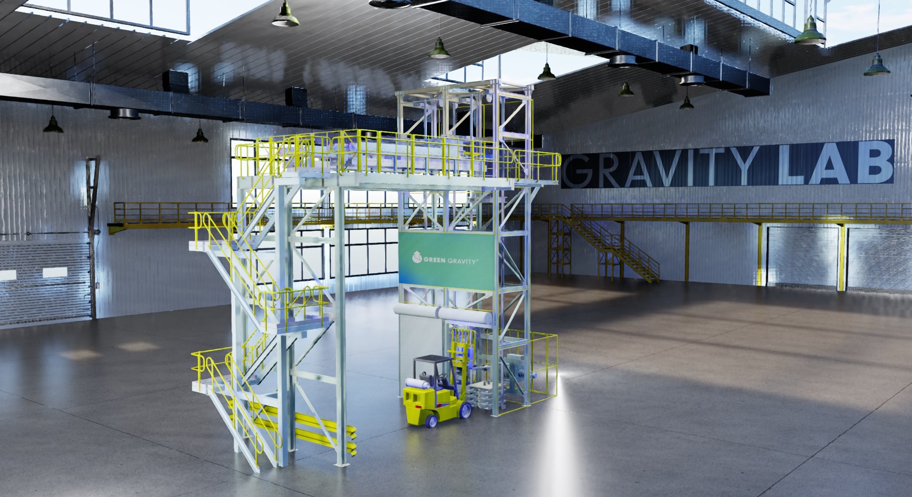
The CEO of startup Green Gravity is prototyping his ambitious vision in a warehouse 60 miles south of Sydney, Australia, and simulating it in NVIDIA Omniverse, a platform for building 3D workflows and applications.
The concept requires some heavy lifting. Solar and wind energy will pull steel blocks weighing as much as 30 cars each up shafts taller than a New York skyscraper, storing potential energy that can turn turbines whenever needed.
A Distributed Energy Network
Swinnerton believes it’s the optimal way to save renewable energy because nearly a million abandoned mine shafts are scattered around the globe, many of them already connected to the grid. And his mechanical system is cheaper and greener than alternatives like massive lithium batteries better suited for electric vehicles.

Officials in Australia, India and the U.S. are interested in the concept, and a state-owned mine operator in Romania is conducting a joint study with Green Gravity.
“We have a tremendous opportunity for repurposing a million mines,” said Swinnerton, who switched gears after a 20-year career at BHP Group, one of the world’s largest mining companies, determined to combat climate change.
A Digital-First Design
A longtime acquaintance saw an opportunity to accelerate Swinnerton’s efforts with a digital twin.
“I was fascinated by the Green Gravity idea and suggested taking a digital-first approach, using data as a differentiator,” said Daniel Keys, an IT expert and executive at xAmplify, a provider of accelerated computing services.
AI-powered simulations could speed the design and deployment of the novel concept, said Keys, who met Swinnerton 25 years earlier at one of their first jobs, flipping burgers at a fast-food stand.
Today, they’ve got a digital prototype cooking on xAmplify’s Scaile computer, based on NVIDIA DGX systems. It’s already accelerating Green Gravity’s proof of concept.
“Thanks to what we inferred with a digital twin, we’ve been able to save 40% of the costs of our physical prototype by shifting from three weights to two and moving them 10 instead of 15 meters vertically,” said Swinnerton.
Use Cases Enabled by Omniverse
It’s the first of many use cases Green Gravity is developing in Omniverse.
Once the prototype is done, the simulation will help scale the design to mines as deep as 7,000 feet, or about six Empire State Buildings stacked on top of each other. Ultimately, the team will build in Omniverse a dashboard to control and monitor sensor-studded facilities without the safety hazards of sending a person into the mine.
“We expect to cut tens of millions of dollars off the estimated $100 million for the first site because we can use simulations to lower our risks with banks and insurers,” said Swinnerton. “That’s a real tantalizing opportunity.”
Virtual Visualization Tools
Operators will track facilities remotely using visualization systems equipped with NVIDIA A40 GPUs and can stream their visuals to tablets thanks to the TabletAR extension in the Omniverse Spatial Framework.
xAmplify’s workflow uses a number of software components such as NVIDIA Modulus, a framework for physics-informed machine learning models.
“We also use Omniverse as a core integration fabric that lets us connect a half-dozen third-party tools operators and developers need, like Siemens PLM for sensor management and Autodesk for design,” Keys said.
Omniverse eases the job of integrating third-party applications into one 3D workflow because it’s based on the OpenUSD standard.
Along the way, AI sifts reams of data about the thousands of available mines to select optimal sites, predicting their potential for energy storage. Machine learning will also help optimize designs for each site.
Taken together, it’s a digital pathway Swinnerton believes will lead to commercial operations for Green Gravity within the next couple years.
It’s the latest customer for xAmplify’s Canberra data center serving Australian government agencies, national defense contractors and an expanding set of enterprise users with a full stack of NVIDIA accelerated software.
Learn more about how AI is transforming renewables, including wind farm optimization, solar energy generation and fusion energy.