Monthly Archives: April 2024

In Part 1 of this series, we presented a solution that used the Amazon Titan Multimodal Embeddings model to convert individual slides from a slide deck into embeddings. We stored the embeddings in a vector database and then used the Large Language-and-Vision Assistant (LLaVA 1.5-7b) model to generate text responses to user questions based on the most similar slide retrieved from the vector database. We used AWS services including Amazon Bedrock, Amazon SageMaker, and Amazon OpenSearch Serverless in this solution.

In this post, we demonstrate a different approach. We use the Anthropic Claude 3 Sonnet model to generate text descriptions for each slide in the slide deck. These descriptions are then converted into text embeddings using the Amazon Titan Text Embeddings model and stored in a vector database. Then we use the Claude 3 Sonnet model to generate answers to user questions based on the most relevant text description retrieved from the vector database.

You can test both approaches for your dataset and evaluate the results to see which approach gives you the best results. In Part 3 of this series, we evaluate the results of both methods.

Solution overview

The solution provides an implementation for answering questions using information contained in text and visual elements of a slide deck. The design relies on the concept of Retrieval Augmented Generation (RAG). Traditionally, RAG has been associated with textual data that can be processed by large language models (LLMs). In this series, we extend RAG to include images as well. This provides a powerful search capability to extract contextually relevant content from visual elements like tables and graphs along with text.

This solution includes the following components:

• Amazon Titan Text Embeddings is a text embeddings model that converts natural language text, including single words, phrases, or even large documents, into numerical representations that can be used to power use cases such as search, personalization, and clustering based on semantic similarity.
• Claude 3 Sonnet is the next generation of state-of-the-art models from Anthropic. Sonnet is a versatile tool that can handle a wide range of tasks, from complex reasoning and analysis to rapid outputs, as well as efficient search and retrieval across vast amounts of information.
• OpenSearch Serverless is an on-demand serverless configuration for Amazon OpenSearch Service. We use OpenSearch Serverless as a vector database for storing embeddings generated by the Amazon Titan Text Embeddings model. An index created in the OpenSearch Serverless collection serves as the vector store for our RAG solution.
• Amazon OpenSearch Ingestion (OSI) is a fully managed, serverless data collector that delivers data to OpenSearch Service domains and OpenSearch Serverless collections. In this post, we use an OSI pipeline API to deliver data to the OpenSearch Serverless vector store.

The solution design consists of two parts: ingestion and user interaction. During ingestion, we process the input slide deck by converting each slide into an image, generating descriptions and text embeddings for each image. We then populate the vector data store with the embeddings and text description for each slide. These steps are completed prior to the user interaction steps.

In the user interaction phase, a question from the user is converted into text embeddings. A similarity search is run on the vector database to find a text description corresponding to a slide that could potentially contain answers to the user question. We then provide the slide description and the user question to the Claude 3 Sonnet model to generate an answer to the query. All the code for this post is available in the GitHub repo.

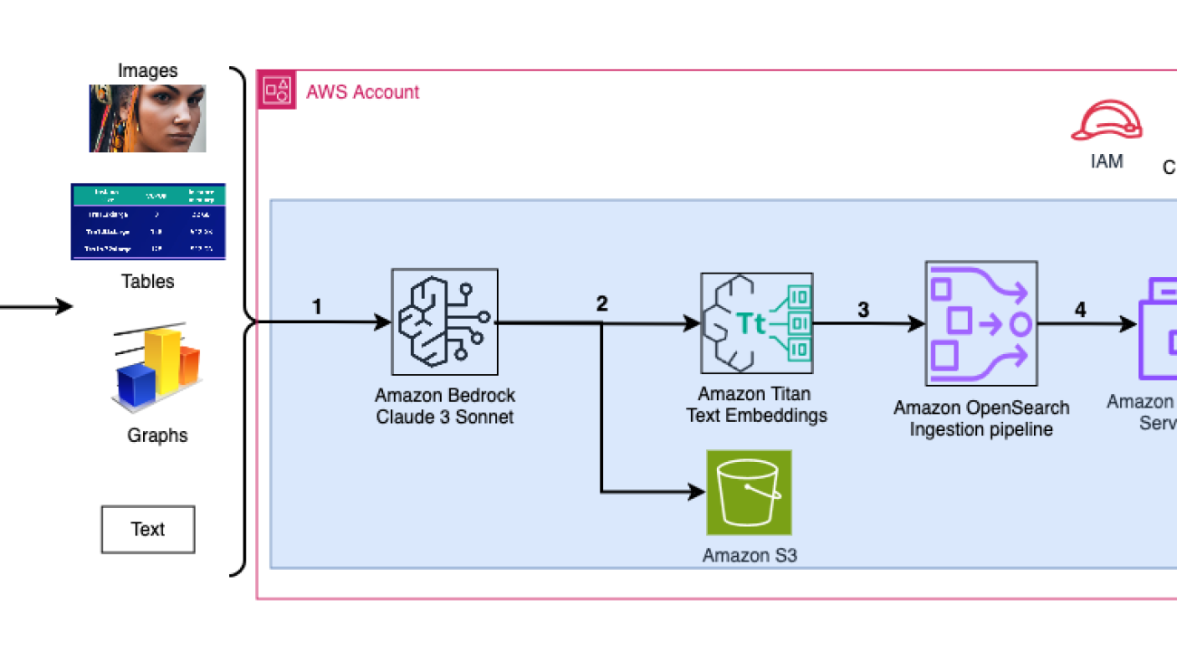
The following diagram illustrates the ingestion architecture.

The workflow consists of the following steps:

1. Slides are converted to image files (one per slide) in JPG format and passed to the Claude 3 Sonnet model to generate text description.
2. The data is sent to the Amazon Titan Text Embeddings model to generate embeddings. In this series, we use the slide deck Train and deploy Stable Diffusion using AWS Trainium & AWS Inferentia from the AWS Summit in Toronto, June 2023 to demonstrate the solution. The sample deck has 31 slides, therefore we generate 31 sets of vector embeddings, each with 1536 dimensions. We add additional metadata fields to perform rich search queries using OpenSearch’s powerful search capabilities.
3. The embeddings are ingested into an OSI pipeline using an API call.
4. The OSI pipeline ingests the data as documents into an OpenSearch Serverless index. The index is configured as the sink for this pipeline and is created as part of the OpenSearch Serverless collection.

The following diagram illustrates the user interaction architecture.

The workflow consists of the following steps:

1. A user submits a question related to the slide deck that has been ingested.
2. The user input is converted into embeddings using the Amazon Titan Text Embeddings model accessed using Amazon Bedrock. An OpenSearch Service vector search is performed using these embeddings. We perform a k-nearest neighbor (k-NN) search to retrieve the most relevant embeddings matching the user query.
3. The metadata of the response from OpenSearch Serverless contains a path to the image and description corresponding to the most relevant slide.
4. A prompt is created by combining the user question and the image description. The prompt is provided to Claude 3 Sonnet hosted on Amazon Bedrock.
5. The result of this inference is returned to the user.

We discuss the steps for both stages in the following sections, and include details about the output.

Prerequisites

To implement the solution provided in this post, you should have an AWS account and familiarity with FMs, Amazon Bedrock, SageMaker, and OpenSearch Service.

This solution uses the Claude 3 Sonnet and Amazon Titan Text Embeddings models hosted on Amazon Bedrock. Make sure that these models are enabled for use by navigating to the Model access page on the Amazon Bedrock console.

If models are enabled, the Access status will state Access granted.

If the models are not available, enable access by choosing Manage model access, selecting the models, and choosing Request model access. The models are enabled for use immediately.

Use AWS CloudFormation to create the solution stack

You can use AWS CloudFormation to create the solution stack. If you have created the solution for Part 1 in the same AWS account, be sure to delete that before creating this stack.

AWS Region	Link
us-east-1
us-west-2

After the stack is created successfully, navigate to the stack’s Outputs tab on the AWS CloudFormation console and note the values for MultimodalCollectionEndpoint and OpenSearchPipelineEndpoint. You use these in the subsequent steps.

The CloudFormation template creates the following resources:

• IAM roles – The following AWS Identity and Access Management (IAM) roles are created. Update these roles to apply least-privilege permissions, as discussed in Security best practices.
  • SMExecutionRole with Amazon Simple Storage Service (Amazon S3), SageMaker, OpenSearch Service, and Amazon Bedrock full access.
  • OSPipelineExecutionRole with access to the S3 bucket and OSI actions.
• SageMaker notebook – All code for this post is run using this notebook.
• OpenSearch Serverless collection – This is the vector database for storing and retrieving embeddings.
• OSI pipeline – This is the pipeline for ingesting data into OpenSearch Serverless.
• S3 bucket – All data for this post is stored in this bucket.

The CloudFormation template sets up the pipeline configuration required to configure the OSI pipeline with HTTP as source and the OpenSearch Serverless index as sink. The SageMaker notebook 2_data_ingestion.ipynb displays how to ingest data into the pipeline using the Requests HTTP library.

The CloudFormation template also creates network, encryption and data access policies required for your OpenSearch Serverless collection. Update these policies to apply least-privilege permissions.

The CloudFormation template name and OpenSearch Service index name are referenced in the SageMaker notebook 3_rag_inference.ipynb. If you change the default names, make sure you update them in the notebook.

Test the solution

After you have created the CloudFormation stack, you can test the solution. Complete the following steps:

1. On the SageMaker console, choose Notebooks in the navigation pane.
2. Select MultimodalNotebookInstance and choose Open JupyterLab.
3. In File Browser, traverse to the notebooks folder to see notebooks and supporting files.

The notebooks are numbered in the sequence in which they run. Instructions and comments in each notebook describe the actions performed by that notebook. We run these notebooks one by one.

4. Choose 1_data_prep.ipynb to open it in JupyterLab.
5. On the Run menu, choose Run All Cells to run the code in this notebook.

This notebook will download a publicly available slide deck, convert each slide into the JPG file format, and upload these to the S3 bucket.

6. Choose 2_data_ingestion.ipynb to open it in JupyterLab.
7. On the Run menu, choose Run All Cells to run the code in this notebook.

In this notebook, you create an index in the OpenSearch Serverless collection. This index stores the embeddings data for the slide deck. See the following code:

session = boto3.Session()
credentials = session.get_credentials()
auth = AWSV4SignerAuth(credentials, g.AWS_REGION, g.OS_SERVICE)

os_client = OpenSearch(
  hosts = [{'host': host, 'port': 443}],
  http_auth = auth,
  use_ssl = True,
  verify_certs = True,
  connection_class = RequestsHttpConnection,
  pool_maxsize = 20
)

index_body = """
{
  "settings": {
    "index.knn": true
  },
  "mappings": {
    "properties": {
      "vector_embedding": {
        "type": "knn_vector",
        "dimension": 1536,
        "method": {
          "name": "hnsw",
          "engine": "nmslib",
          "parameters": {}
        }
      },
      "image_path": {
        "type": "text"
      },
      "slide_text": {
        "type": "text"
      },
      "slide_number": {
        "type": "text"
      },
      "metadata": { 
        "properties" :
          {
            "filename" : {
              "type" : "text"
            },
            "desc":{
              "type": "text"
            }
          }
      }
    }
  }
}
"""
index_body = json.loads(index_body)
try:
  response = os_client.indices.create(index_name, body=index_body)
  logger.info(f"response received for the create index -> {response}")
except Exception as e:
  logger.error(f"error in creating index={index_name}, exception={e}")

You use the Claude 3 Sonnet and Amazon Titan Text Embeddings models to convert the JPG images created in the previous notebook into vector embeddings. These embeddings and additional metadata (such as the S3 path and description of the image file) are stored in the index along with the embeddings. The following code snippet shows how Claude 3 Sonnet generates image descriptions:

def get_img_desc(image_file_path: str, prompt: str):
    # read the file, MAX image size supported is 2048 * 2048 pixels
    with open(image_file_path, "rb") as image_file:
        input_image_b64 = image_file.read().decode('utf-8')
  
    body = json.dumps(
        {
            "anthropic_version": "bedrock-2023-05-31",
            "max_tokens": 1000,
            "messages": [
                {
                    "role": "user",
                    "content": [
                        {
                            "type": "image",
                            "source": {
                                "type": "base64",
                                "media_type": "image/jpeg",
                                "data": input_image_b64
                            },
                        },
                        {"type": "text", "text": prompt},
                    ],
                }
            ],
        }
    )
    
    response = bedrock.invoke_model(
        modelId=g.CLAUDE_MODEL_ID,
        body=body
    )

    resp_body = json.loads(response['body'].read().decode("utf-8"))
    resp_text = resp_body['content'][0]['text'].replace('"', "'")

    return resp_text

The image descriptions are passed to the Amazon Titan Text Embeddings model to generate vector embeddings. These embeddings and additional metadata (such as the S3 path and description of the image file) are stored in the index along with the embeddings. The following code snippet shows the call to the Amazon Titan Text Embeddings model:

def get_text_embedding(bedrock: botocore.client, prompt_data: str) -> np.ndarray:
    body = json.dumps({
        "inputText": prompt_data,
    })    
    try:
        response = bedrock.invoke_model(
            body=body, modelId=g.TITAN_MODEL_ID, accept=g.ACCEPT_ENCODING, contentType=g.CONTENT_ENCODING
        )
        response_body = json.loads(response['body'].read())
        embedding = response_body.get('embedding')
    except Exception as e:
        logger.error(f"exception={e}")
        embedding = None

    return embedding

The data is ingested into the OpenSearch Serverless index by making an API call to the OSI pipeline. The following code snippet shows the call made using the Requests HTTP library:

data = json.dumps([{
    "image_path": input_image_s3, 
    "slide_text": resp_text, 
    "slide_number": slide_number, 
    "metadata": {
        "filename": obj_name, 
        "desc": "" 
    }, 
    "vector_embedding": embedding
}])

r = requests.request(
    method='POST', 
    url=osi_endpoint, 
    data=data,
    auth=AWSSigV4('osis'))

8. Choose 3_rag_inference.ipynb to open it in JupyterLab.
9. On the Run menu, choose Run All Cells to run the code in this notebook.

This notebook implements the RAG solution: you convert the user question into embeddings, find a similar image description from the vector database, and provide the retrieved description to Claude 3 Sonnet to generate an answer to the user question. You use the following prompt template:

  llm_prompt: str = """

  Human: Use the summary to provide a concise answer to the question to the best of your abilities. If you cannot answer the question from the context then say I do not know, do not make up an answer.
  <question>
  {question}
  </question>

  <summary>
  {summary}
  </summary>

  Assistant:"""

The following code snippet provides the RAG workflow:

def get_llm_response(bedrock: botocore.client, question: str, summary: str) -> str:
    prompt = llm_prompt.format(question=question, summary=summary)
    
    body = json.dumps(
    {
        "anthropic_version": "bedrock-2023-05-31",
        "max_tokens": 1000,
        "messages": [
            {
                "role": "user",
                "content": [
                    {"type": "text", "text": prompt},
                ],
            }
        ],
    })
        
    try:
        response = bedrock.invoke_model(
        modelId=g.CLAUDE_MODEL_ID,
        body=body)

        response_body = json.loads(response['body'].read().decode("utf-8"))
        llm_response = response_body['content'][0]['text'].replace('"', "'")
        
    except Exception as e:
        logger.error(f"exception while slide_text={summary[:10]}, exception={e}")
        llm_response = None

    return llm_response

# create prompt and convert to embeddings question: str = "How does Inf2 compare in performance to comparable EC2 instances? I need numbers." text_embedding = get_text_embedding(bedrock, question) # vector db search vector_db_response: Dict = find_similar_data(text_embeddings) # download image for local notebook display s3_img_path = vector_db_response.get('hits', {}).get('hits')[0].get('_source').get('image_path') logger.info(f"going to answer the question="{question}" using the image "{s3_img_path}"") !aws s3 cp {s3_img_path} . local_img_path = os.path.basename(s3_img_path) display(filename=local_img_path) # Ask Claude 3 Sonnet slide_text = vector_db_response.get('hits', {}).get('hits')[0].get('_source').get('slide_text') llm_response = get_llm_response(bedrock, question, slide_text) print(llm_response)

Results

The following table contains some user questions and responses generated by our implementation. The Question column captures the user question, and the Answer column is the textual response generated by Claude 3 Sonnet. The Image column shows the k-NN slide match returned by the OpenSearch Serverless vector search.

Multimodal RAG results

Question	Answer	Image
How does Inf2 compare in performance to comparable EC2 instances? I need numbers.	Based on the information provided in the summary, the key performance comparison numbers given for the Amazon EC2 Inf2 instances compared to other instances are: 1. Up to 4x higher throughput. 2. Up to 10x lower latency. The summary does not provide specific numbers comparing the Inf2 instances to other EC2 instance types. However, it highlights the throughput and latency improvements as the main performance advantages of the Inf2 instances over comparable instances for running generative AI models.
As per the AI/ML flywheel, what do the AWS AI/ML services provide?	Based on the summary, the AWS AI/ML services provide a range of capabilities that fuel an AI/ML flywheel. This flywheel consists of innovation in developing new and better algorithms, enabling more use-cases and applications, driving wider adoption and demand, which in turn leads to further investment in research and optimization to drive more innovation. The AWS AI/ML services seem to offer the tools, resources, and infrastructure to support this continuous cycle of innovation, application development, adoption, and reinvestment in the field of artificial intelligence and machine learning.
Compared to GPT-2, how many more parameters does GPT-3 have? What is the numerical difference between the parameter size of GPT-2 and GPT-3?	According to the information provided in the summary, GPT-3 from 2020 had 175B (175 billion) parameters, while GPT-2 from 2019 had 1.5B (1.5 billion) parameters. Therefore, the numerical difference between the parameter size of GPT-2 and GPT-3 is 173.5 billion parameters. GPT-3 has approximately 115 times more parameters than GPT-2.
What are quarks in particle physics?	Unfortunately, the given summary does not contain any information about quarks in particle physics. The summary describes an image related to the progression of natural language processing and generative AI technologies, but it does not mention anything about particle physics or the concept of quarks.

Query your index

You can use OpenSearch Dashboards to interact with the OpenSearch API to run quick tests on your index and ingested data.

Cleanup

To avoid incurring future charges, delete the resources. You can do this by deleting the stack using the AWS CloudFormation console.

Conclusion

Enterprises generate new content all the time, and slide decks are a common way to share and disseminate information internally within the organization and externally with customers or at conferences. Over time, rich information can remain buried and hidden in non-text modalities like graphs and tables in these slide decks.

You can use this solution and the power of multimodal FMs such as the Amazon Titan Text Embeddings and Claude 3 Sonnet to discover new information or uncover new perspectives on content in slide decks. You can try different Claude models available on Amazon Bedrock by updating the CLAUDE_MODEL_ID in the globals.py file.

This is Part 2 of a three-part series. We used the Amazon Titan Multimodal Embeddings and the LLaVA model in Part 1. In Part 3, we will compare the approaches from Part 1 and Part 2.

Portions of this code are released under the Apache 2.0 License.

About the authors

Amit Arora is an AI and ML Specialist Architect at Amazon Web Services, helping enterprise customers use cloud-based machine learning services to rapidly scale their innovations. He is also an adjunct lecturer in the MS data science and analytics program at Georgetown University in Washington D.C.

Manju Prasad is a Senior Solutions Architect at Amazon Web Services. She focuses on providing technical guidance in a variety of technical domains, including AI/ML. Prior to joining AWS, she designed and built solutions for companies in the financial services sector and also for a startup. She is passionate about sharing knowledge and fostering interest in emerging talent.

Archana Inapudi is a Senior Solutions Architect at AWS, supporting a strategic customer. She has over a decade of cross-industry expertise leading strategic technical initiatives. Archana is an aspiring member of the AI/ML technical field community at AWS. Prior to joining AWS, Archana led a migration from traditional siloed data sources to Hadoop at a healthcare company. She is passionate about using technology to accelerate growth, provide value to customers, and achieve business outcomes.

Antara Raisa is an AI and ML Solutions Architect at Amazon Web Services, supporting strategic customers based out of Dallas, Texas. She also has previous experience working with large enterprise partners at AWS, where she worked as a Partner Success Solutions Architect for digital-centered customers.

Read More

This is a guest post co-written with the leadership team of Iambic Therapeutics.

Iambic Therapeutics is a drug discovery startup with a mission to create innovative AI-driven technologies to bring better medicines to cancer patients, faster.

Our advanced generative and predictive artificial intelligence (AI) tools enable us to search the vast space of possible drug molecules faster and more effectively. Our technologies are versatile and applicable across therapeutic areas, protein classes, and mechanisms of action. Beyond creating differentiated AI tools, we have established an integrated platform that merges AI software, cloud-based data, scalable computation infrastructure, and high-throughput chemistry and biology capabilities. The platform both enables our AI—by supplying data to refine our models—and is enabled by it, capitalizing on opportunities for automated decision-making and data processing.

We measure success by our ability to produce superior clinical candidates to address urgent patient need, at unprecedented speed: we advanced from program launch to clinical candidates in just 24 months, significantly faster than our competitors.

In this post, we focus on how we used Karpenter on Amazon Elastic Kubernetes Service (Amazon EKS) to scale AI training and inference, which are core elements of the Iambic discovery platform.

The need for scalable AI training and inference

Every week, Iambic performs AI inference across dozens of models and millions of molecules, serving two primary use cases:

• Medicinal chemists and other scientists use our web application, Insight, to explore chemical space, access and interpret experimental data, and predict properties of newly designed molecules. All of this work is done interactively in real time, creating a need for inference with low latency and medium throughput.
• At the same time, our generative AI models automatically design molecules targeting improvement across numerous properties, searching millions of candidates, and requiring enormous throughput and medium latency.

Guided by AI technologies and expert drug hunters, our experimental platform generates thousands of unique molecules each week, and each is subjected to multiple biological assays. The generated data points are automatically processed and used to fine-tune our AI models every week. Initially, our model fine-tuning took hours of CPU time, so a framework for scaling model fine-tuning on GPUs was imperative.

Our deep learning models have non-trivial requirements: they are gigabytes in size, are numerous and heterogeneous, and require GPUs for fast inference and fine-tuning. Looking to cloud infrastructure, we needed a system that allows us to access GPUs, scale up and down quickly to handle spiky, heterogeneous workloads, and run large Docker images.

We wanted to build a scalable system to support AI training and inference. We use Amazon EKS and were looking for the best solution to auto scale our worker nodes. We chose Karpenter for Kubernetes node auto scaling for a number of reasons:

• Ease of integration with Kubernetes, using Kubernetes semantics to define node requirements and pod specs for scaling
• Low-latency scale-out of nodes
• Ease of integration with our infrastructure as code tooling (Terraform)

The node provisioners support effortless integration with Amazon EKS and other AWS resources such as Amazon Elastic Compute Cloud (Amazon EC2) instances and Amazon Elastic Block Store volumes. The Kubernetes semantics used by the provisioners support directed scheduling using Kubernetes constructs such as taints or tolerations and affinity or anti-affinity specifications; they also facilitate control over the number and types of GPU instances that may be scheduled by Karpenter.

Solution overview

In this section, we present a generic architecture that is similar to the one we use for our own workloads, which allows elastic deployment of models using efficient auto scaling based on custom metrics.

The following diagram illustrates the solution architecture.

The architecture deploys a simple service in a Kubernetes pod within an EKS cluster. This could be a model inference, data simulation, or any other containerized service, accessible by HTTP request. The service is exposed behind a reverse-proxy using Traefik. The reverse proxy collects metrics about calls to the service and exposes them via a standard metrics API to Prometheus. The Kubernetes Event Driven Autoscaler (KEDA) is configured to automatically scale the number of service pods, based on the custom metrics available in Prometheus. Here we use the number of requests per second as a custom metric. The same architectural approach applies if you choose a different metric for your workload.

Karpenter monitors for any pending pods that can’t run due to lack of sufficient resources in the cluster. If such pods are detected, Karpenter adds more nodes to the cluster to provide the necessary resources. Conversely, if there are more nodes in the cluster than what is needed by the scheduled pods, Karpenter removes some of the worker nodes and the pods get rescheduled, consolidating them on fewer instances. The number of HTTP requests per second and number of nodes can be visualized using a Grafana dashboard. To demonstrate auto scaling, we run one or more simple load-generating pods, which send HTTP requests to the service using curl.

Solution deployment

In the step-by-step walkthrough, we use AWS Cloud9 as an environment to deploy the architecture. This enables all steps to be completed from a web browser. You can also deploy the solution from a local computer or EC2 instance.

To simplify deployment and improve reproducibility, we follow the principles of the do-framework and the structure of the depend-on-docker template. We clone the aws-do-eks project and, using Docker, we build a container image that is equipped with the necessary tooling and scripts. Within the container, we run through all the steps of the end-to-end walkthrough, from creating an EKS cluster with Karpenter to scaling EC2 instances.

For the example in this post, we use the following EKS cluster manifest:

apiVersion: eksctl.io/v1alpha5
kind: ClusterConfig
metadata:
  name: do-eks-yaml-karpenter
version: '1.28'
region: us-west-2
tags:
  karpenter.sh/discovery: do-eks-yaml-karpenter
iam:
  withOIDC: true
addons:
  - name: aws-ebs-csi-driver
    version: v1.26.0-eksbuild.1
wellKnownPolicies:
  ebsCSIController: true
managedNodeGroups:
  - name: c5-xl-do-eks-karpenter-ng
    instanceType: c5.xlarge
    instancePrefix: c5-xl
    privateNetworking: true
    minSize: 0
    desiredCapacity: 2
    maxSize: 10
    volumeSize: 300
    iam:
      withAddonPolicies:
        cloudWatch: true
        ebs: true

This manifest defines a cluster named do-eks-yaml-karpenter with the EBS CSI driver installed as an add-on. A managed node group with two c5.xlarge nodes is included to run system pods that are needed by the cluster. The worker nodes are hosted in private subnets, and the cluster API endpoint is public by default.

You could also use an existing EKS cluster instead of creating one. We deploy Karpenter by following the instructions in the Karpenter documentation, or by running the following script, which automates the deployment instructions.

The following code shows the Karpenter configuration we use in this example:

apiVersion: karpenter.sh/v1beta1
kind: NodePool
metadata:
  name: default
spec:
  template:
    metadata: null
    labels:
      cluster-name: do-eks-yaml-karpenter
    annotations:
      purpose: karpenter-example
    spec:
      nodeClassRef:
        apiVersion: karpenter.k8s.aws/v1beta1
        kind: EC2NodeClass
        name: default
        requirements:
          - key: karpenter.sh/capacity-type
            operator: In
            values:
              - spot
              - on-demand
          - key: karpenter.k8s.aws/instance-category
            operator: In
            values:
              - c
              - m
              - r
              - g
              - p
          - key: karpenter.k8s.aws/instance-generation
            operator: Gt
            values:
              - '2'
  disruption:
    consolidationPolicy: WhenUnderutilized
    #consolidationPolicy: WhenEmpty
    #consolidateAfter: 30s
    expireAfter: 720h
---
apiVersion: karpenter.k8s.aws/v1beta1
kind: EC2NodeClass
metadata:
  name: default
spec:
  amiFamily: AL2
  subnetSelectorTerms:
    - tags:
      karpenter.sh/discovery: "do-eks-yaml-karpenter"
  securityGroupSelectorTerms:
    - tags:
      karpenter.sh/discovery: "do-eks-yaml-karpenter"
  role: "KarpenterNodeRole-do-eks-yaml-karpenter"
  tags:
    app: autoscaling-test
  blockDeviceMappings:
    - deviceName: /dev/xvda
      ebs:
        volumeSize: 80Gi
        volumeType: gp3
        iops: 10000
        deleteOnTermination: true
        throughput: 125
  detailedMonitoring: true

We define a default Karpenter NodePool with the following requirements:

• Karpenter can launch instances from both spot and on-demand capacity pools
• Instances must be from the “c” (compute optimized), “m” (general purpose), “r” (memory optimized), or “g” and “p” (GPU accelerated) computing families
• Instance generation must be greater than 2; for example, g3 is acceptable, but g2 is not

The default NodePool also defines disruption policies. Underutilized nodes will be removed so pods can be consolidated to run on fewer or smaller nodes. Alternatively, we can configure empty nodes to be removed after the specified time period. The expireAfter setting specifies the maximum lifetime of any node, before it is stopped and replaced if necessary. This helps reduce security vulnerabilities as well as avoid issues that are typical for nodes with long uptimes, such as file fragmentation or memory leaks.

By default, Karpenter provisions nodes with a small root volume, which can be insufficient for running AI or machine learning (ML) workloads. Some of the deep learning container images can be tens of GB in size, and we need to make sure there is enough storage space on the nodes to run pods using these images. To do that, we define EC2NodeClass with blockDeviceMappings, as shown in the preceding code.

Karpenter is responsible for auto scaling at the cluster level. To configure auto scaling at the pod level, we use KEDA to define a custom resource called ScaledObject, as shown in the following code:

apiVersion: keda.sh/v1alpha1
kind: ScaledObject
metadata:
  name: keda-prometheus-hpa
  namespace: hpa-example
spec:
  scaleTargetRef:
    name: php-apache
  minReplicaCount: 1
  cooldownPeriod: 30
  triggers:
    - type: prometheus
      metadata:
        serverAddress: http://prometheus- server.prometheus.svc.cluster.local:80
        metricName: http_requests_total
        threshold: '1'
        query: rate(traefik_service_requests_total{service="hpa-example-php-apache-80@kubernetes",code="200"}[2m])

The preceding manifest defines a ScaledObject named keda-prometheus-hpa, which is responsible for scaling the php-apache deployment and always keeps at least one replica running. It scales the pods of this deployment based on the metric http_requests_total available in Prometheus obtained by the specified query, and targets to scale up the pods so that each pod serves no more than one request per second. It scales down the replicas after the request load has been below the threshold for longer than 30 seconds.

The deployment spec for our example service contains the following resource requests and limits:

resources:
  limits:
    cpu: 500m
    nvidia.com/gpu: 1
  requests:
    cpu: 200m
    nvidia.com/gpu: 1

With this configuration, each of the service pods will use exactly one NVIDIA GPU. When new pods are created, they will be in Pending state until a GPU is available. Karpenter adds GPU nodes to the cluster as needed to accommodate the pending pods.

A load-generating pod sends HTTP requests to the service with a pre-set frequency. We increase the number of requests by increasing the number of replicas in the load-generator deployment.

A full scaling cycle with utilization-based node consolidation is visualized in a Grafana dashboard. The following dashboard shows the number of nodes in the cluster by instance type (top), the number of requests per second (bottom left), and the number of pods (bottom right).

We start with just the two c5.xlarge CPU instances that the cluster was created with. Then we deploy one service instance, which requires a single GPU. Karpenter adds a g4dn.xlarge instance to accommodate this need. We then deploy the load generator, which causes KEDA to add more service pods and Karpenter adds more GPU instances. After optimization, the state settles on one p3.8xlarge instance with 8 GPUs and one g5.12xlarge instance with 4 GPUs.

When we scale the load-generating deployment to 40 replicas, KEDA creates additional service pods to maintain the required request load per pod. Karpenter adds g4dn.metal and g4dn.12xlarge nodes to the cluster to provide the needed GPUs for the additional pods. In the scaled state, the cluster contains 16 GPU nodes and serves about 300 requests per second. When we scale down the load generator to 1 replica, the reverse process takes place. After the cooldown period, KEDA reduces the number of service pods. Then as fewer pods run, Karpenter removes the underutilized nodes from the cluster and the service pods get consolidated to run on fewer nodes. When the load generator pod is removed, a single service pod on a single g4dn.xlarge instance with 1 GPU remains running. When we remove the service pod as well, the cluster is left in the initial state with only two CPU nodes.

We can observe this behavior when the NodePool has the setting consolidationPolicy: WhenUnderutilized.

With this setting, Karpenter dynamically configures the cluster with as few nodes as possible, while providing sufficient resources for all pods to run and also minimizing cost.

The scaling behavior shown in the following dashboard is observed when the NodePool consolidation policy is set to WhenEmpty, along with consolidateAfter: 30s.

In this scenario, nodes are stopped only when there are no pods running on them after the cool-off period. The scaling curve appears smooth, compared to the utilization-based consolidation policy; however, it can be seen that more nodes are used in the scaled state (22 vs. 16).

Overall, combining pod and cluster auto scaling makes sure that the cluster scales dynamically with the workload, allocating resources when needed and removing them when not in use, thereby maximizing utilization and minimizing cost.

Outcomes

Iambic used this architecture to enable efficient use of GPUs on AWS and migrate workloads from CPU to GPU. By using EC2 GPU powered instances, Amazon EKS, and Karpenter, we were able to enable faster inference for our physics-based models and fast experiment iteration times for applied scientists who rely on training as a service.

The following table summarizes some of the time metrics of this migration.

The following table summarizes some of our time and cost metrics.

Summary

In this post, we showcased how Iambic used Karpenter and KEDA to scale our Amazon EKS infrastructure to meet the latency requirements of our AI inference and training workloads. Karpenter and KEDA are powerful open source tools that help auto scale EKS clusters and workloads running on them. This helps optimize compute costs while meeting performance requirements. You can check out the code and deploy the same architecture in your own environment by following the complete walkthrough in this GitHub repo.

About the Authors

Matthew Welborn is the director of Machine Learning at Iambic Therapeutics. He and his team leverage AI to accelerate the identification and development of novel therapeutics, bringing life-saving medicines to patients faster.

Paul Whittemore is a Principal Engineer at Iambic Therapeutics. He supports delivery of the infrastructure for the Iambic AI-driven drug discovery platform.

Alex Iankoulski is a Principal Solutions Architect, ML/AI Frameworks, who focuses on helping customers orchestrate their AI workloads using containers and accelerated computing infrastructure on AWS.

Read More

Migrating to the cloud is an essential step for modern organizations aiming to capitalize on the flexibility and scale of cloud resources. Tools like Terraform and AWS CloudFormation are pivotal for such transitions, offering infrastructure as code (IaC) capabilities that define and manage complex cloud environments with precision. However, despite its benefits, IaC’s learning curve, and the complexity of adhering to your organization’s and industry-specific compliance and security standards, could slow down your cloud adoption journey. Organizations typically counter these hurdles by investing in extensive training programs or hiring specialized personnel, which often leads to increased costs and delayed migration timelines.

Generative artificial intelligence (AI) with Amazon Bedrock directly addresses these challenges. Amazon Bedrock is a fully managed service that offers a choice of high-performing foundation models (FMs) from leading AI companies like AI21 Labs, Anthropic, Cohere, Meta, Stability AI, and Amazon with a single API, along with a broad set of capabilities to build generative AI applications with security, privacy, and responsible AI. Amazon Bedrock empowers teams to generate Terraform and CloudFormation scripts that are custom fitted to organizational needs while seamlessly integrating compliance and security best practices. Traditionally, cloud engineers learning IaC would manually sift through documentation and best practices to write compliant IaC scripts. With Amazon Bedrock, teams can input high-level architectural descriptions and use generative AI to generate a baseline configuration of Terraform scripts. These generated scripts are tailored to meet your organization’s unique requirements while conforming to industry standards for security and compliance. These scripts serve as a foundational starting point, requiring further refinement and validation to make sure they meet production-level standards.

This solution not only accelerates the migration process but also provides a standardized and secure cloud infrastructure. Additionally, it offers beginner cloud engineers initial script drafts as standard templates to build upon, facilitating their IaC learning journey.

As you navigate the complexities of cloud migration, the need for a structured, secure, and compliant environment is paramount. AWS Landing Zone addresses this need by offering a standardized approach to deploying AWS resources. This makes sure your cloud foundation is built according to AWS best practices from the start. With AWS Landing Zone, you eliminate the guesswork in security configurations, resource provisioning, and account management. It’s particularly beneficial for organizations looking to scale without compromising on governance or control, providing a clear path to a robust and efficient cloud setup.

In this post, we show you how to generate customized, compliant IaC scripts for AWS Landing Zone using Amazon Bedrock.

AWS Landing Zone architecture in the context of cloud migration

AWS Landing Zone can help you set up a secure, multi-account AWS environment based on AWS best practices. It provides a baseline environment to get started with a multi-account architecture, automate the setup of new accounts, and centralize compliance, security, and identity management. The following is an example of a customized Terraform-based AWS Landing Zone solution, in which each application resides in its own AWS account.

The high-level workflow includes the following components:

• Module provisioning – Different platform teams across various domains, such as databases, containers, data management, networking, and security, develop and publish certified or custom modules. These are delivered through pipelines to a Terraform private module registry, which is maintained by the organization for consistency and standardization.
• Account vending machine layer – The account vending machine (AVM) layer uses either AWS Control Tower, AWS Account Factory for Terraform (AFT), or a custom landing zone solution to vend accounts. In this post, we refer to these solutions collectively as the AVM layer. When application owners submit a request to the AVM layer, it processes the input parameters from the request to provision a target AWS account. This account is then provisioned with tailored infrastructure components through AVM customizations, which include AWS Control Tower customizations or AFT customizations.
• Application infrastructure layer – In this layer, application teams deploy their infrastructure components into the provisioned AWS accounts. This is achieved by writing Terraform code within an application-specific repository. The Terraform code calls upon the modules previously published to the Terraform private registry by the platform teams.

Overcoming on-premises IaC migration challenges with generative AI

Teams maintaining on-premises applications often encounter a learning curve with Terraform, a key tool for IaC in AWS environments. This skill gap can be a significant hurdle in cloud migration efforts. Amazon Bedrock, with its generative AI capabilities, plays an essential role in mitigating this challenge. It facilitates the automation of Terraform code creation for the application infrastructure layer, empowering teams with limited Terraform experience to make an efficient transition to AWS.

Amazon Bedrock generates Terraform code from architectural descriptions. The generated code is custom and standardized based on organizational best practices, security, and regulatory guidelines. This standardization is made possible by using advanced prompts in conjunction with Knowledge Bases for Amazon Bedrock, which stores information on organization-specific Terraform modules. This solution uses Retrieval Augmented Generation (RAG) to enrich the input prompt to Amazon Bedrock with details from the knowledge base, making sure the output Terraform configuration and README contents are compliant with your organization’s Terraform best practices and guidelines.

The following diagram illustrates this architecture.

The workflow consists of the following steps:

1. The process begins with account vending, where application owners submit a request for a new AWS account. This invokes the AVM, which processes the request parameters to provision the target AWS account.
2. An architecture description for an application slated for migration is passed as one of the inputs to the AVM layer.
3. After the account is provisioned, AVM customizations are applied. This can include AWS Control Tower customizations or AFT customizations that set up the account with the necessary infrastructure components and configurations in line with organizational policies.
4. In parallel, the AVM layer invokes a Lambda function to generate Terraform code. This function enriches the architecture description with a customized prompt, and utilizes RAG to further enhance the prompt with organization-specific coding guidelines from the Knowledge Base for Bedrock. This Knowledge Base includes tailored best practices, security guardrails, and guidelines specific to the organization. See an illustrative example of organization specific Terraform module specifications and  guidelines uploaded to the Knowledge Base.
5. Before deployment, the initial draft of the Terraform code is thoroughly reviewed by cloud engineers or an automated code review system to confirm that it meets all technical and compliance standards.
6. The reviewed and updated Terraform scripts are then used to deploy infrastructure components into the newly provisioned AWS account, setting up compute, storage, and networking resources required for the application.

Solution overview

The AWS Landing Zone deployment uses a Lambda function for generating Terraform scripts from architectural inputs. This function, which is central to the operation, translates these inputs into compliant code, using Amazon Bedrock and Knowledge Bases for Amazon Bedrock. The output is then stored in a GitHub repository, corresponding to the specific application in migration. The following sections detail the prerequisites and specific steps needed to implement this solution.

Prerequisites

You should have the following:

• An AWS account with appropriate AWS Identity and Access Management (IAM) permissions to create Lambda functions, Amazon Simple Storage Service (Amazon S3) buckets, IAM roles, and other resources.
• A GitHub account with a repository to store the generated Terraform scripts.
• Access to Amazon Bedrock models. For more information, refer to Model access.

Configure the Lambda function to generate custom code

This Lambda function is a key component in automating the creation of customized, compliant Terraform configurations for AWS services. It commits the generated configurations directly to a designated GitHub repository, aligning with organizational best practices. For the function code, refer to the following GitHub repo. For creating lambda function, please follow instructions.

The following diagram illustrates the workflow of the function.

The workflow includes the following steps:

1. The function is invoked by an event from the AVM layer, containing the architecture description.
2. The function retrieves and uses Terraform module definitions from the knowledge base.
3. The function invokes the Amazon Bedrock model twice, following recommended prompt engineering guidelines. The function applies RAG to enrich the input prompt with the Terraform module information, making sure the output code meets organizational best practices.
   • First, generate Terraform configurations following organizational coding guidelines and include Terraform module details from the knowledge base. For example, the prompt could be: “Generate Terraform configurations for AWS services. Follow security best practices by using IAM roles and least privilege permissions. Include all necessary parameters, with default values. Add comments explaining the overall architecture and the purpose of each resource.”
   • Second, create a detailed README file. For example: “Generate a detailed README for the Terraform configuration based on AWS services. Include sections on security improvements, cost optimization tips following the AWS Well-Architected Framework. Also, include detailed Cost Breakdown for each AWS service used with hourly rates and total daily and monthly costs.”
4. It commits the generated Terraform configuration and the README to the GitHub repository, providing traceability and transparency.
5. Lastly, it responds with success, including URLs to the committed GitHub files, or returns detailed error information for troubleshooting.

Configure Knowledge Bases for Amazon Bedrock

Follow these steps to set up your knowledge base in Amazon Bedrock:

1. On the Amazon Bedrock console, choose Knowledge base in the navigation pane.
2. Choose Create knowledge base.
3. Enter a clear and descriptive name that reflects the purpose of your knowledge base, such as AWS Account Setup Knowledge Base For Amazon Bedrock.
4. Assign a pre-configured IAM role with the necessary permissions. It’s typically best to let Amazon Bedrock create this role for you to make sure it has the correct permissions.
5. Upload a JSON file to an S3 bucket with encryption enabled for security. This file should contain a structured list of AWS services and Terraform modules. For the JSON structure, use the following example from the GitHub repository.
6. Choose the default embeddings model.
7. Allow Amazon Bedrock to create and manage the vector store for you in Amazon OpenSearch Service.
8. Review the information for accuracy. Pay special attention to the S3 bucket URI and IAM role details.
9. Create your knowledge base.

After you deploy and configure these components, when your AWS Landing Zone solution invokes the Lambda function, the following files are generated:

• A Terraform configuration file – This file specifies the infrastructure setup.
• A comprehensive README file – This file documents the security standards embedded within the code, confirming that they align with the security practices outlined in the initial sections. Additionally, this README includes an architectural summary, cost optimization tips, and a detailed cost breakdown for the resources described in the Terraform configuration.

The following screenshot shows an example of the Terraform configuration file.

The following screenshot shows an example of the README file.

Clean up

Complete the following steps to clean up your resources:

1. Delete the Lambda function if it’s no longer required.
2. Empty and delete the S3 bucket used for Terraform state storage.
3. Remove the generated Terraform scripts and README file from the GitHub repo.
4. Delete the knowledge base if it’s no longer needed.

Conclusion

The generative AI capabilities of Amazon Bedrock not only streamline the creation of compliant Terraform scripts for AWS deployments, but also act as a pivotal learning aid for beginner cloud engineers transitioning on-premises applications to AWS. This approach accelerates the cloud migration process and helps you adhere to best practices. You can also use the solution to provide value after the migration, enhancing daily operations such as ongoing infrastructure and cost optimization. Although we primarily focused on Terraform in this post, these principles can also enhance your AWS CloudFormation deployments, providing a versatile solution for your infrastructure needs.

Ready to simplify your cloud migration process with generative AI in Amazon Bedrock? Begin by exploring the Amazon Bedrock User Guide to understand how it can streamline your organization’s cloud journey. For further assistance and expertise, consider using AWS Professional Services to help you streamline your cloud migration journey and maximize the benefits of Amazon Bedrock.

Unlock the potential for rapid, secure, and efficient cloud adoption with Amazon Bedrock. Take the first step today and discover how it can enhance your organization’s cloud transformation endeavors.

About the Author

Ebbey Thomas specializes in strategizing and developing custom AWS Landing Zone resources with a focus on using generative AI to enhance cloud infrastructure automation. In his role at AWS Professional Services, Ebbey’s expertise is central to architecting solutions that streamline cloud adoption, providing a secure and efficient operational framework for AWS users. He is known for his innovative approach to cloud challenges and his commitment to driving forward the capabilities of cloud services.

Read More