DeepSeek-R1, developed by AI startup DeepSeek AI, is an advanced large language model (LLM) distinguished by its innovative, multi-stage training process. Instead of relying solely on traditional pre-training and fine-tuning, DeepSeek-R1 integrates reinforcement learning to achieve more refined outputs. The model employs a chain-of-thought (CoT) approach that systematically breaks down complex queries into clear, logical steps. Additionally, it uses NVIDIA’s parallel thread execution (PTX) constructs to boost training efficiency, and a combined framework of supervised fine-tuning (SFT) and group robust policy optimization (GRPO) makes sure its results are both transparent and interpretable.
In this post, we demonstrate how to optimize hosting DeepSeek-R1 distilled models with Hugging Face Text Generation Inference (TGI) on Amazon SageMaker AI.
Model Variants
The current DeepSeek model collection consists of the following models:
- DeepSeek-V3 – An LLM that uses a Mixture-of-Experts (MoE) architecture. MoE models like DeepSeek-V3 and Mixtral replace the standard feed-forward neural network in transformers with a set of parallel sub-networks called experts. These experts are selectively activated for each input, allowing the model to efficiently scale to a much larger size without a corresponding increase in computational cost. For example, DeepSeek-V3 is a 671-billion-parameter model, but only 37 billion parameters (approximately 5%) are activated during the output of each token. DeepSeek-V3-Base is the base model from which the R1 variants are derived.
- DeepSeek-R1-Zero – A fine-tuned variant of DeepSeek-V3 based on using reinforcement learning to guide CoT reasoning capabilities, without any SFT done prior. According to the DeepSeek R1 paper, DeepSeek-R1-Zero excelled at reasoning behaviors but encountered challenges with readability and language mixing.
- DeepSeek-R1 – Another fine-tuned variant of DeepSeek-V3-Base, built similarly to DeepSeek-R1-Zero, but with a multi-step training pipeline. DeepSeek-R1 starts with a small amount of cold-start data prior to the GRPO process. It also incorporates SFT data through rejection sampling, combined with supervised data generated from DeepSeek-V3 to retrain DeepSeek-V3-base. After this, the retrained model goes through another round of RL, resulting in the DeepSeek-R1 model checkpoint.
- DeepSeek-R1-Distill – Variants of Hugging Face’s Qwen and Meta’s Llama based on Qwen2.5-Math-1.5B, Qwen2.5-Math-7B, Qwen2.5-14B, Qwen2.5-32B, Llama-3.1-8B, and Llama-3.3-70B-Instruct. The distilled model variants are a result of fine-tuning Qwen or Llama models through knowledge distillation, where DeepSeek-R1 acts as the teacher and Qwen or Llama as the student. These models retain their existing architecture while gaining additional reasoning capabilities through a distillation process. They are exclusively fine-tuned using SFT and don’t incorporate any RL techniques.
The following figure illustrates the performance of DeepSeek-R1 compared to other state-of-the-art models on standard benchmark tests, such as MATH-500, MMLU, and more.

Hugging Face Text Generation Inference (TGI)
Hugging Face Text Generation Inference (TGI) is a high-performance, production-ready inference framework optimized for deploying and serving large language models (LLMs) efficiently. It is designed to handle the demanding computational and latency requirements of state-of-the-art transformer models, including Llama, Falcon, Mistral, Mixtral, and GPT variants – for a full list of TGI supported models refer to supported models.
Amazon SageMaker AI provides a managed way to deploy TGI-optimized models, offering deep integration with Hugging Face’s inference stack for scalable and cost-efficient LLM deployment. To learn more about Hugging Face TGI support on Amazon SageMaker AI, refer to this announcement post and this documentation on deploy models to Amazon SageMaker AI.
Key Optimizations in Hugging Face TGI
Hugging Face TGI is built to address the challenges associated with deploying large-scale text generation models, such as inference latency, token throughput, and memory constraints.
The benefits of using TGI include:
- Tensor parallelism – Splits large models across multiple GPUs for efficient memory utilization and computation
- Continuous batching – Dynamically batches multiple inference requests to maximize token throughput and reduce latency
- Quantization – Lowers memory usage and computational cost by converting model weights to INT8 or FP16
- Speculative decoding – Uses a smaller draft model to speed up token prediction while maintaining accuracy
- Key-value cache optimization – Reduces redundant computations for faster response times in long-form text generation
- Token streaming – Streams tokens in real time for low-latency applications like chatbots and virtual assistants
Runtime TGI Arguments
TGI containers support runtime configurations that provide greater control over LLM deployments. These configurations allow you to adjust settings such as quantization, model parallel size (tensor parallel size), maximum tokens, data type (dtype), and more using container environment variables.
Notable runtime parameters influencing your model deployment include:
HF_MODEL_ID : This parameter specifies the identifier of the model to load, which can be a model ID from the Hugging Face Hub (e.g., meta-llama/Llama-3.2-11B-Vision-Instruct) or Simple Storage Service (S3) URI containing the model files.HF_TOKEN : This parameter variable provides the access token required to download gated models from the Hugging Face Hub, such as Llama or Mistral.SM_NUM_GPUS : This parameter specifies the number of GPUs to use for model inference, allowing the model to be sharded across multiple GPUs for improved performance.MAX_CONCURRENT_REQUESTS : This parameter controls the maximum number of concurrent requests that the server can handle, effectively managing the load and ensuring optimal performance.DTYPE : This parameter sets the data type for the model weights during loading, with options like float16 or bfloat16, influencing the model’s memory consumption and computational performance.
There are additional optional runtime parameters that are already pre-optimized in TGI containers to maximize performance on host hardware. However, you can modify them to exercise greater control over your LLM inference performance:
MAX_TOTAL_TOKENS: This parameter sets the upper limit on the combined number of input and output tokens a deployment can handle per request, effectively defining the “memory budget” for client interactions.MAX_INPUT_TOKENS : This parameter specifies the maximum number of tokens allowed in the input prompt of each request, controlling the length of user inputs to manage memory usage and ensure efficient processing.MAX_BATCH_PREFILL_TOKENS : This parameter caps the total number of tokens processed during the prefill stage across all batched requests, a phase that is both memory-intensive and compute-bound, thereby optimizing resource utilization and preventing out-of-memory errors.
For a complete list of runtime configurations, please refer to text-generation-launcher arguments.
DeepSeek Deployment Patterns with TGI on Amazon SageMaker AI
Amazon SageMaker AI offers a simple and streamlined approach to deploy DeepSeek-R1 models with just a few lines of code. Additionally, SageMaker endpoints support automatic load balancing and autoscaling, enabling your LLM deployment to scale dynamically based on incoming requests. During non-peak hours, the endpoint can scale down to zero, optimizing resource usage and cost efficiency.
The table below summarizes all DeepSeek-R1 models available on the Hugging Face Hub, as uploaded by the original model provider, DeepSeek.
DeepSeek AI also offers distilled versions of its DeepSeek-R1 model to offer more efficient alternatives for various applications.
There are two ways to deploy LLMs, such as DeepSeek-R1 and its distilled variants, on Amazon SageMaker:
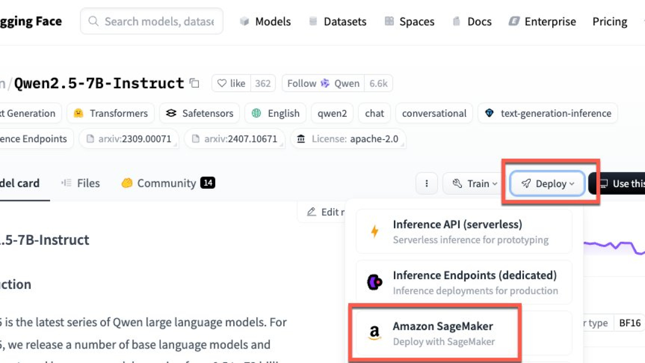
Option 1: Direct Deployment from Hugging Face Hub
The easiest way to host DeepSeek-R1 in your AWS account is by deploying it (along with its distilled variants) using TGI containers. These containers simplify deployment through straightforward runtime environment specifications. The architecture diagram below shows a direct download from the Hugging Face Hub, ensuring seamless integration with Amazon SageMaker.
The following code shows how to deploy the DeepSeek-R1-Distill-Llama-8B model to a SageMaker endpoint, directly from the Hugging Face Hub.
import sagemaker
from sagemaker.huggingface import (
    HuggingFaceModel,
    get_huggingface_llm_image_uri
)

role = sagemaker.get_execution_role()
session = sagemaker.Session()

# select the latest 3+ version container
deploy_image_uri = get_huggingface_llm_image_uri(
     "huggingface",
     version="3.0.1"
)

deepseek_tgi_model = HuggingFaceModel(
            image_uri=deploy_image_uri,
    env={
        "HF_MODEL_ID": "deepseek-ai/DeepSeek-R1-Distill-Llama-8B",
        "ENDPOINT_SERVER_TIMEOUT": "3600",
        ...
    },
    role=role,
    sagemaker_session=session,
    name="deepseek-r1-llama-8b-model" # optional
)

pretrained_tgi_predictor = deepseek_tgi_model.deploy(
   endpoint_name="deepseek-r1-llama-8b-endpoint", # optional
    initial_instance_count=1,
    instance_type="ml.g5.2xlarge",
    container_startup_health_check_timeout=600,
    wait=False, # set to true to wait for endpoint InService
)
To deploy other distilled models, simply update the HF_MODEL_ID to any of the DeepSeek distilled model variants, such as deepseek-ai/DeepSeek-R1-Distill-Qwen-1.5B, deepseek-ai/DeepSeek-R1-Distill-Qwen-32B, or deepseek-ai/DeepSeek-R1-Distill-Llama-70B.
Option 2: Deployment from a Private S3 Bucket
To deploy models privately within your AWS account, upload the DeepSeek-R1 model weights to a S3 bucket and set HF_MODEL_ID to the corresponding S3 bucket prefix. TGI will then retrieve and deploy the model weights from S3, eliminating the need for internet downloads during each deployment. This approach reduces model loading latency by keeping the weights closer to your SageMaker endpoints and enable your organization’s security teams to perform vulnerability scans before deployment. SageMaker endpoints also support auto-scaling, allowing DeepSeek-R1 to scale horizontally based on incoming request volume while seamlessly integrating with elastic load balancing.
Deploying a DeepSeek-R1 distilled model variant from S3 follows the same process as option 1, with one key difference: HF_MODEL_ID points to the S3 bucket prefix instead of the Hugging Face Hub. Before deployment, you must first download the model weights from the Hugging Face Hub and upload them to your S3 bucket.
deepseek_tgi_model = HuggingFaceModel(
            image_uri=deploy_image_uri,
    env={
        "HF_MODEL_ID": "s3://my-model-bucket/path/to/model",
        ...
    },
          vpc_config={
                 "Subnets": ["subnet-xxxxxxxx", "subnet-yyyyyyyy"],
    "SecurityGroupIds": ["sg-zzzzzzzz"]
     },
    role=role,
    sagemaker_session=session,
    name="deepseek-r1-llama-8b-model-s3" # optional
)
Deployment Best Practices
The following are some best practices to consider when deploying DeepSeek-R1 models on SageMaker AI:
- Deploy within a private VPC – It’s recommended to deploy your LLM endpoints inside a virtual private cloud (VPC) and behind a private subnet, preferably with no egress. See the following code:
deepseek_tgi_model = HuggingFaceModel(
            image_uri=deploy_image_uri,
    env={
        "HF_MODEL_ID": "deepseek-ai/DeepSeek-R1-Distill-Llama-8B",
        "ENDPOINT_SERVER_TIMEOUT": "3600",
        ...
    },
    role=role,
          vpc_config={
                 "Subnets": ["subnet-xxxxxxxx", "subnet-yyyyyyyy"],
                 "SecurityGroupIds": ["sg-zzzzzzzz"]
     },
    sagemaker_session=session,
    name="deepseek-r1-llama-8b-model" # optional
)
- Implement guardrails for safety and compliance – Always apply guardrails to validate incoming and outgoing model responses for safety, bias, and toxicity. You can use Amazon Bedrock Guardrails to enforce these protections on your SageMaker endpoint responses.
Inference Performance Evaluation
This section presents examples of the inference performance of DeepSeek-R1 distilled variants on Amazon SageMaker AI. Evaluating LLM performance across key metrics—end-to-end latency, throughput, and resource efficiency—is crucial for ensuring responsiveness, scalability, and cost-effectiveness in real-world applications. Optimizing these metrics directly enhances user experience, system reliability, and deployment feasibility at scale.
All DeepSeek-R1 Qwen (1.5B, 7B, 14B, 32B) and Llama (8B, 70B) variants are evaluated against four key performance metrics:
- End-to-End Latency
- Throughput (Tokens per Second)
- Time to First Token
- Inter-Token Latency
Please note that the main purpose of this performance evaluation is to give you an indication about relative performance of distilled R1 models on different hardware. We didn’t try to optimize the performance for each model/hardware/use case combination. These results should not be treated like a best possible performance of a particular model on a particular instance type. You should always perform your own testing using your own datasets and input/output sequence length.
If you are interested in running this evaluation job inside your own account, refer to our code on GitHub.
Scenarios
We tested the following scenarios:
- Tokens – Two input token lengths were used to evaluate the performance of DeepSeek-R1 distilled variants hosted on SageMaker endpoints. Each test was executed 100 times, with concurrency set to 1, and the average values across key performance metrics were recorded. All models were run with dtype=bfloat16.
- Short-length test – 512 input tokens, 256 output tokens.
- Medium-length test – 3,072 input tokens, 256 output tokens.
- Hardware – Several instance families were tested, including p4d (NVIDIA A100), g5 (NVIDIA A10G), g6 (NVIDIA L4), and g6e (NVIDIA L40s), each equipped with 1, 4, or 8 GPUs per instance. For additional details regarding pricing and instance specifications, refer to Amazon SageMaker AI pricing. In the following table, a green cell indicates a model was tested on a specific instance type, and a red cell indicates the model wasn’t tested because the instance type or size was excessive for the model or unable to run because of insufficient GPU memory.

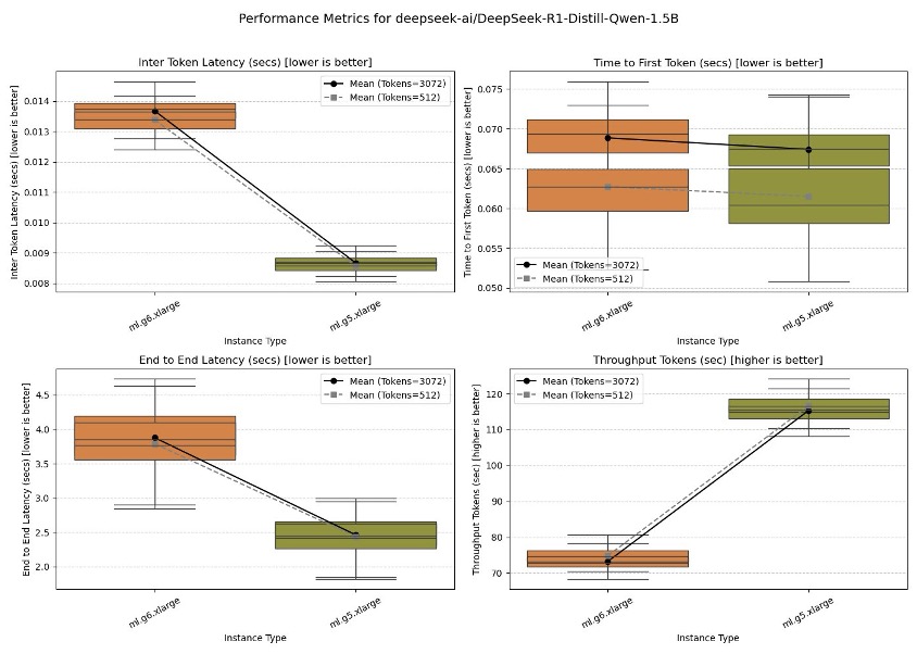
In the following sections we use a box plot to visualize model performance. A box is a concise visual summary that displays a dataset’s median, interquartile range (IQR), and potential outliers using a box for the middle 50% of the data with whiskers extending to the smallest and largest non-outlier values. By examining the median’s placement within the box, the box’s size, and the whiskers’ lengths, you can quickly assess the data’s central tendency, variability, and skewness.

DeepSeek-R1-Distill-Qwen-1.5B
A single GPU instance is sufficient to host one or multiple concurrent DeepSeek-R1-Distill-Qwen-1.5B serving workers on TGI. In this test, a single worker was deployed, and performance was evaluated across the four outlined metrics. Results show that the ml.g5.xlarge outperforms the ml.g6.xlarge across all metrics.
DeepSeek-R1-Distill-Qwen-7B
DeepSeek-R1-Distill-Qwen-7B was tested on ml.g5.xlarge, ml.g5.2xlarge, ml.g6.xlarge, ml.g6.2xlarge, and ml.g6e.xlarge. The ml.g6e.xlarge instance performed the best, followed by ml.g5.2xlarge, ml.g5.xlarge, and the ml.g6 instances.

DeepSeek-R1-Distill-Llama-8B
Similar to the 7B variant, DeepSeek-R1-Distill-Llama-8B was benchmarked across ml.g5.xlarge, ml.g5.2xlarge, ml.g6.xlarge, ml.g6.2xlarge, and ml.g6e.xlarge, with ml.g6e.xlarge demonstrating the highest performance among all instances.

DeepSeek-R1-Distill-Qwen-14B
DeepSeek-R1-Distill-Qwen-14B was tested on ml.g5.12xlarge, ml.g6.12xlarge, ml.g6e.2xlarge, and ml.g6e.xlarge. The ml.g5.12xlarge exhibited the highest performance, followed by ml.g6.12xlarge. Although at a lower performance profile, DeepSeek-R1-14B can also be deployed on the single GPU g6e instances due to their larger memory footprint.

DeepSeek-R1-Distill-Qwen-32B
DeepSeek-R1-Distill-Qwen-32B requires more than 48GB of memory, making ml.g5.12xlarge, ml.g6.12xlarge, and ml.g6e.12xlarge suitable for performance comparison. In this test, ml.g6e.12xlarge delivered the highest performance, followed by ml.g5.12xlarge, with ml.g6.12xlarge ranking third.

DeepSeek-R1-Distill-Llama-70B
DeepSeek-R1-Distill-Llama-70B was tested on ml.g5.48xlarge, ml.g6.48xlarge, ml.g6e.12xlarge, ml.g6e.48xlarge, and ml.p4dn.24xlarge. The best performance was observed on ml.p4dn.24xlarge, followed by ml.g6e.48xlarge, ml.g6e.12xlarge, ml.g5.48xlarge, and finally ml.g6.48xlarge.

Clean Up
To avoid incurring cost after completing your evaluation, ensure you delete the endpoints you created earlier.
import boto3

# Create a low-level SageMaker service client.
sagemaker_client = boto3.client('sagemaker', region_name=<region>)

# Delete endpoint
sagemaker_client.delete_endpoint(EndpointName=endpoint_name)
Conclusion
In this blog, you learned about the current versions of DeepSeek models and how to use the Hugging Face TGI containers to simplify the deployment of DeepSeek-R1 distilled models (or any other LLM) on Amazon SageMaker AI to just a few lines of code. You also learned how to deploy models directly from the Hugging Face Hub for quick experimentation and from a private S3 bucket to provide enhanced security and model deployment performance.
Finally, you saw an extensive evaluation of all DeepSeek-R1 distilled models across four key inference performance metrics using 13 different NVIDIA accelerator instance types. This analysis provides valuable insights to help you select the optimal instance type for your DeepSeek-R1 deployment. All code used to analyze DeepSeek-R1 distilled model variants are available on GitHub.
About the Authors
 Pranav Murthy is a Worldwide Technical Lead and Sr. GenAI Data Scientist at AWS. He helps customers build, train, deploy, evaluate, and monitor Machine Learning (ML), Deep Learning (DL), and Generative AI (GenAI) workloads on Amazon SageMaker. Pranav specializes in multimodal architectures, with deep expertise in computer vision (CV) and natural language processing (NLP). Previously, he worked in the semiconductor industry, developing AI/ML models to optimize semiconductor processes using state-of-the-art techniques. In his free time, he enjoys playing chess, training models to play chess, and traveling. You can find Pranav on LinkedIn.
 Simon Pagezy is a Cloud Partnership Manager at Hugging Face, dedicated to making cutting-edge machine learning accessible through open source and open science. With a background in AI/ML consulting at AWS, he helps organizations leverage the Hugging Face ecosystem on their platform of choice.
 Giuseppe Zappia is a Principal AI/ML Specialist Solutions Architect at AWS, focused on helping large enterprises design and deploy ML solutions on AWS. He has over 20 years of experience as a full stack software engineer, and has spent the past 5 years at AWS focused on the field of machine learning.
 Dmitry Soldatkin is a Senior Machine Learning Solutions Architect at AWS, helping customers design and build AI/ML solutions. Dmitry’s work covers a wide range of ML use cases, with a primary interest in generative AI, deep learning, and scaling ML across the enterprise. He has helped companies in many industries, including insurance, financial services, utilities, and telecommunications. He has a passion for continuous innovation and using data to drive business outcomes. Prior to joining AWS, Dmitry was an architect, developer, and technology leader in data analytics and machine learning fields in the financial services industry.
Read More


 Jim Burtoft is a Senior Startup Solutions Architect at AWS and works directly with startups as well as the team at Hugging Face. Jim is a CISSP, part of the AWS AI/ML Technical Field Community, part of the Neuron Data Science community, and works with the open source community to enable the use of Inferentia and Trainium. Jim holds a bachelor’s degree in mathematics from Carnegie Mellon University and a master’s degree in economics from the University of Virginia.
 Miriam Lebowitz is a Solutions Architect focused on empowering early-stage startups at AWS. She leverages her experience with AIML to guide companies to select and implement the right technologies for their business objectives, setting them up for scalable growth and innovation in the competitive startup world.
 Rhia Soni is a Startup Solutions Architect at AWS. Rhia specializes in working with early stage startups and helps customers adopt Inferentia and Trainium. Rhia is also part of the AWS Analytics Technical Field Community and is a subject matter expert in Generative BI. Rhia holds a bachelor’s degree in Information Science from the University of Maryland.
 Paul Aiuto is a Senior Solution Architect Manager focusing on Startups at AWS. Paul created a team of AWS Startup Solution architects that focus on the adoption of Inferentia and Trainium. Paul holds a bachelor’s degree in Computer Science from Siena College and has multiple Cyber Security certifications.


 Carole Suarez is a Senior Solutions Architect at AWS, where she helps guide startups through their cloud journey. Carole specializes in data engineering and holds an array of AWS certifications on a variety of topics including analytics, AI, and security. She is passionate about learning languages and is fluent in English, French, and Tagalog.
 Ben Gruher is a Generative AI Solutions Architect at AWS, focusing on startup customers. Ben graduated from Seattle University where he obtained bachelor’s and master’s degrees in Computer Science and Data Science.
 Harrison Hunter is the CTO and co-founder of MaestroQA where he leads the engineer and product teams. Prior to MaestroQA, Harrison studied computer science and AI at MIT.
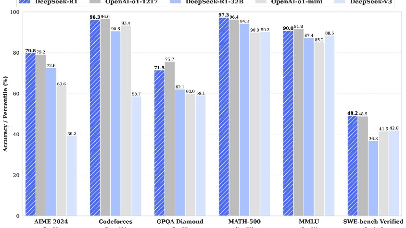
 deepseek-ai/DeepSeek-R1-Zero


 NVIDIA GeForce NOW (@NVIDIAGFN)


 Yanyan Zhang is a Senior Generative AI Data Scientist at Amazon Web Services, where she has been working on cutting-edge AI/ML technologies as a Generative AI Specialist, helping customers use generative AI to achieve their desired outcomes. Yanyan graduated from Texas A&M University with a PhD in Electrical Engineering. Outside of work, she loves traveling, working out, and exploring new things.

 Nitin Eusebius is a Sr. Enterprise Solutions Architect at AWS, experienced in Software Engineering, Enterprise Architecture, and AI/ML. He is deeply passionate about exploring the possibilities of generative AI. He collaborates with customers to help them build well-architected applications on the AWS platform, and is dedicated to solving technology challenges and assisting with their cloud journey.