As businesses and developers increasingly seek to optimize their language models for specific tasks, the decision between model customization and Retrieval Augmented Generation (RAG) becomes critical. In this post, we seek to address this growing need by offering clear, actionable guidelines and best practices on when to use each approach, helping you make informed decisions that align with your unique requirements and objectives.
The introduction of Amazon Nova models represent a significant advancement in the field of AI, offering new opportunities for large language model (LLM) optimization. In this post, we demonstrate how to effectively perform model customization and RAG with Amazon Nova models as a baseline. We conducted a comprehensive comparison study between model customization and RAG using the latest Amazon Nova models, and share these valuable insights.
Approach and base model overview
In this section, we discuss the differences between a fine-tuning and RAG approach, present common use cases for each approach, and provide an overview of the base model used for experiments.
Demystifying RAG and model customization
RAG is a technique to enhance the capability of pre-trained models by allowing the model access to external domain-specific data sources. It combines two components: retrieval of external knowledge and generation of responses. It allows pre-trained language models to dynamically incorporate external data during the response-generation process, enabling more contextually accurate and updated outputs. Unlike fine-tuning, in RAG, the model doesn’t undergo any training and the model weights aren’t updated to learn the domain knowledge. Although fine-tuning implicitly uses domain-specific information by embedding the required knowledge directly into the model, RAG explicitly uses the domain-specific information through external retrieval.
Model customization refers to adapting a pre-trained language model to better fit specific tasks, domains, or datasets. Fine-tuning is one such technique, which helps in injecting task-specific or domain-specific knowledge for improving model performance. It adjusts the model’s parameters to better align with the nuances of the target task while using its general knowledge.
Common use cases for each approach
RAG is optimal for use cases requiring dynamic or frequently updated data (such as customer support FAQs and ecommerce catalogs), domain-specific insights (such as legal or medical Q&A), scalable solutions for broad applications (such as software as a service (SaaS) platforms), multimodal data retrieval (such as document summarization), and strict compliance with secure or sensitive data (such as financial and regulatory systems).
Conversely, fine-tuning thrives in scenarios demanding precise customization (such as personalized chatbots or creative writing), high accuracy for narrow tasks (such as code generation or specialized summarization), ultra-low latency (such as real-time customer interactions), stability with static datasets (such as domain-specific glossaries), and cost-efficient scaling for high-volume tasks (such as call center automation).
Although RAG excels at real-time grounding in external data and fine-tuning specializes in static, structured, and personalized workflows, choosing between them often depends on nuanced factors. This post offers a comprehensive comparison of RAG and fine-tuning, clarifying their strengths, limitations, and contexts where each approach delivers the best performance.
Introduction to Amazon Nova models
Amazon Nova is a new generation of foundation model (FM) offering frontier intelligence and industry-leading price-performance. Amazon Nova Pro and Amazon Nova Lite are multimodal models excelling in accuracy and speed, with Amazon Nova Lite optimized for low-cost, fast processing. Amazon Nova Micro focuses on text tasks with ultra-low latency. They offer fast inference, support agentic workflows with Amazon Bedrock Knowledge Bases and RAG, and allow fine-tuning for text and multi-modal data. Optimized for cost-effective performance, they are trained on data in over 200 languages.
Solution overview
To evaluate the effectiveness of RAG compared to model customization, we designed a comprehensive testing framework using a set of AWS-specific questions. Our study used Amazon Nova Micro and Amazon Nova Lite as baseline FMs and tested their performance across different configurations.
We structured our evaluation as follows:
- Base model:
- Used out-of-box Amazon Nova Micro and Amazon Nova Lite
- Generated responses to AWS-specific questions without additional context
- Base model with RAG:
- Connected the base models to Amazon Bedrock Knowledge Bases
- Provided access to relevant AWS documentation and blogs
- Model customization:
- Fine-tuned both Amazon Nova models using 1,000 AWS-specific question-answer pairs generated from the same set of AWS articles
- Deployed the customized models through provisioned throughput
- Generated responses to AWS-specific questions with fine-tuned models
- Model customization and RAG combined approach:
-
- Connected the fine-tuned models to Amazon Bedrock Knowledge Bases
- Provided fine-tuned models access to relevant AWS articles at inference time
In the following sections, we walk through how to set up the second and third approaches (base model with RAG and model customization with fine-tuning) in Amazon Bedrock.
Prerequisites
To follow along with this post, you need the following prerequisites:
- An AWS account and appropriate permissions
- An Amazon Simple Storage Service (Amazon S3) bucket with two folders: one containing your training data, and one for your model output and training metrics
Implement RAG with the baseline Amazon Nova model
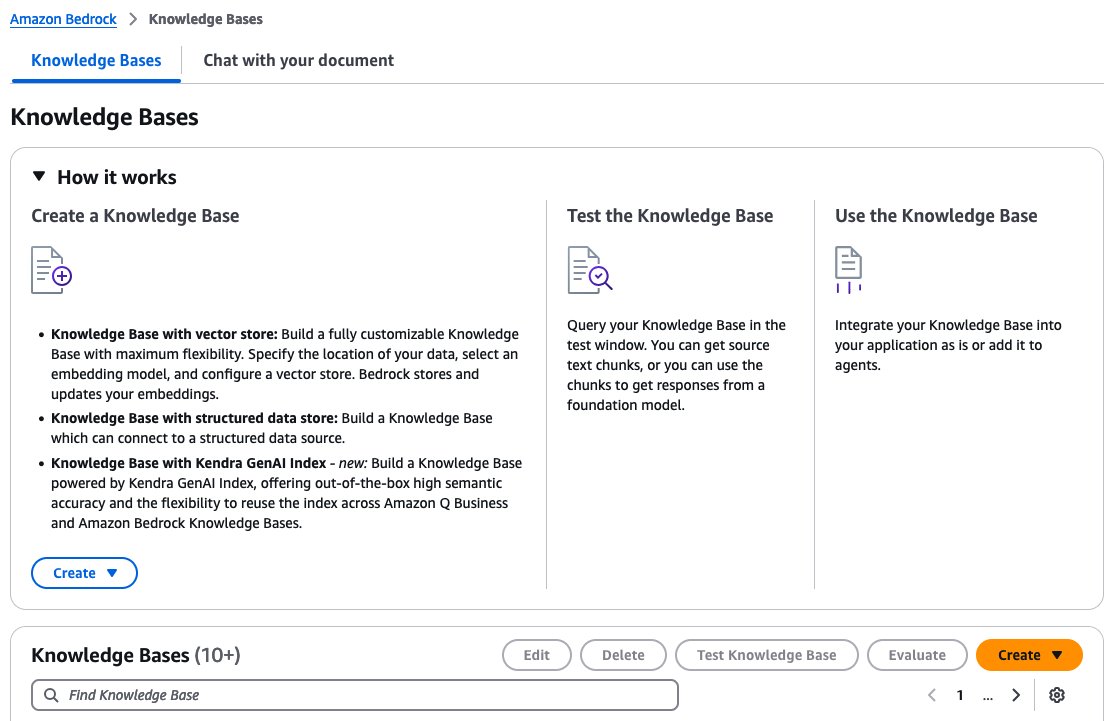
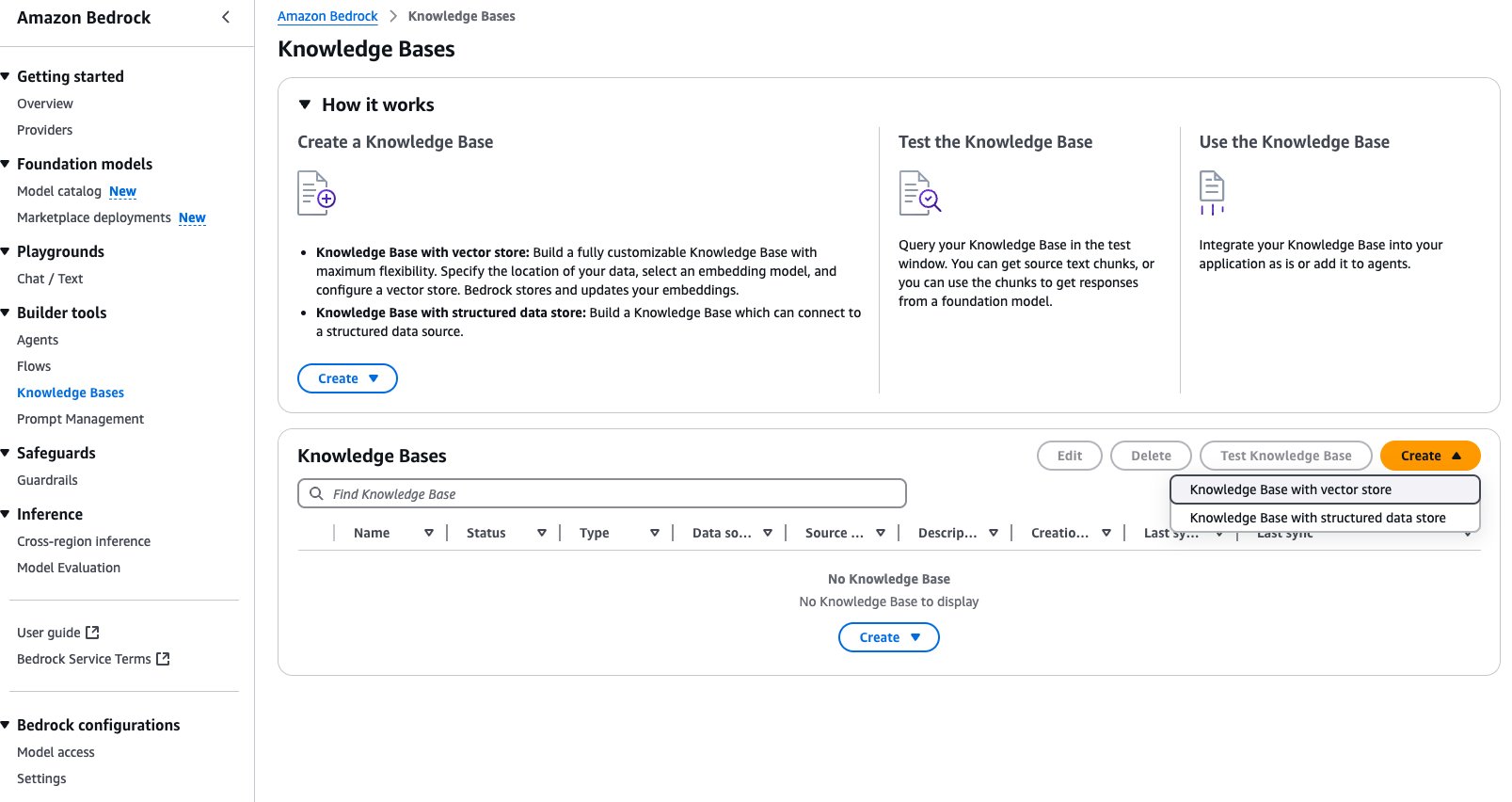
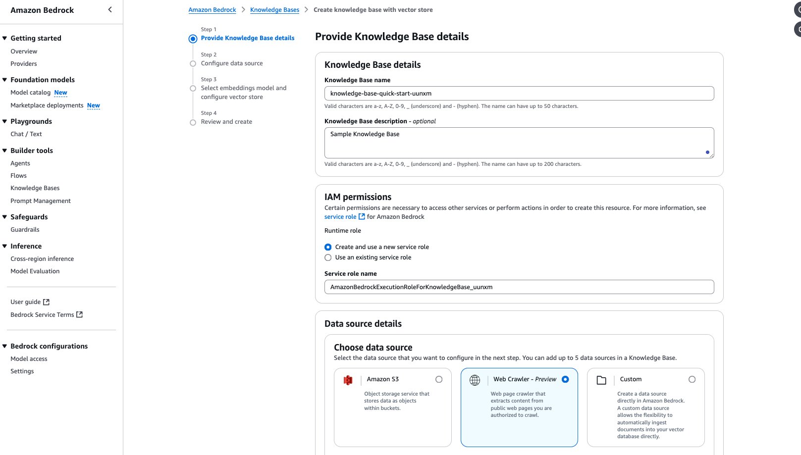
In this section, we walk through the steps to implement RAG with the baseline model. To do so, we create a knowledge base. Complete the following steps:
- On the Amazon Bedrock console, choose Knowledge Bases in the navigation pane.
- Under Knowledge Bases, choose Create.
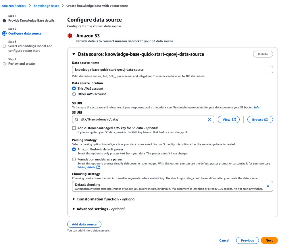
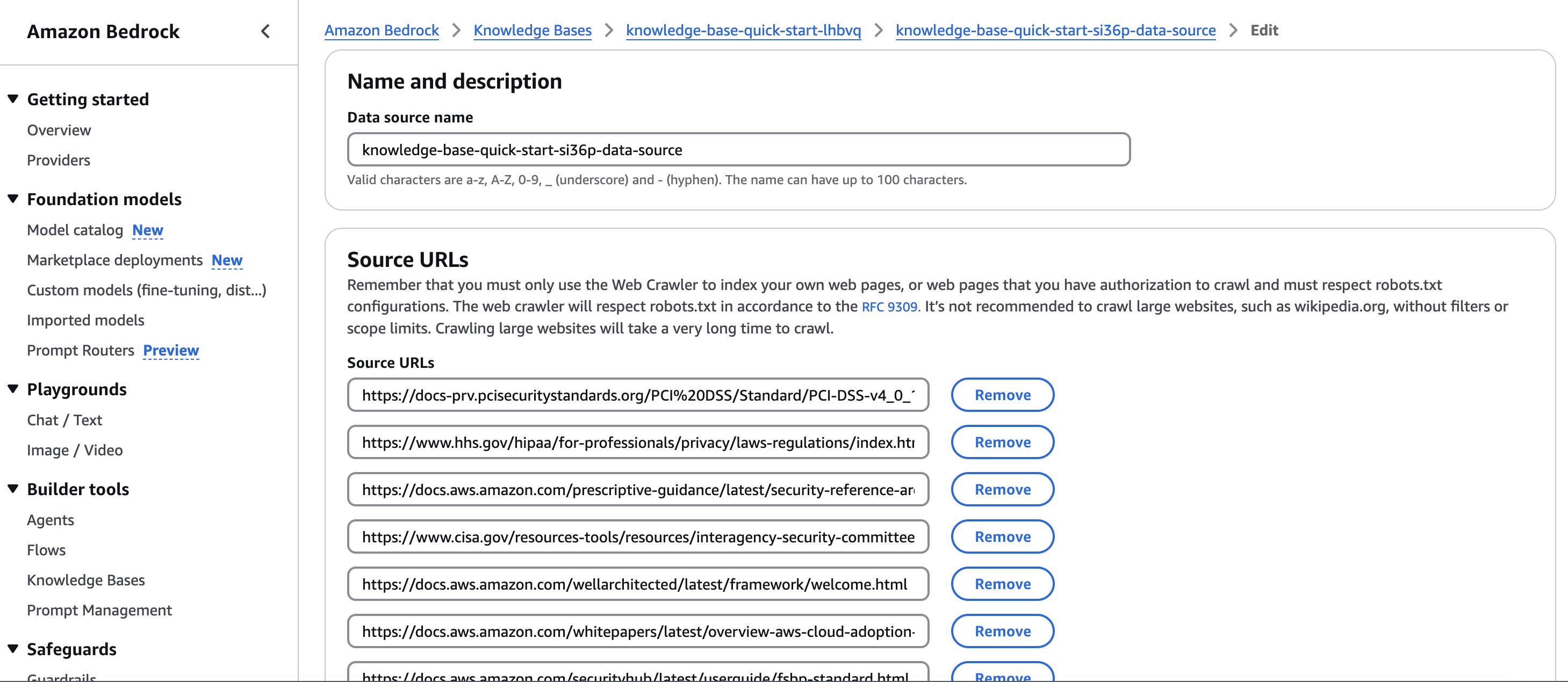
- On the Configure data source page, provide the following information:
- Specify the Amazon S3 location of the documents.
- Specify a chunking strategy.
- Choose Next.
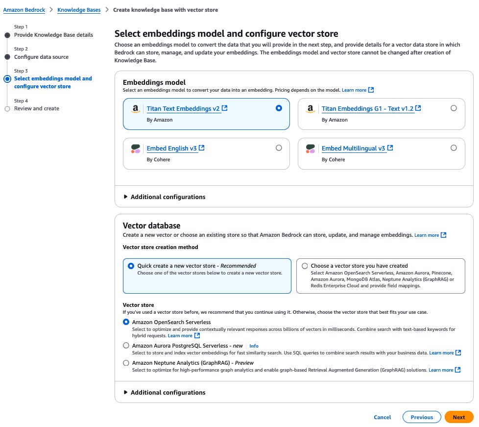
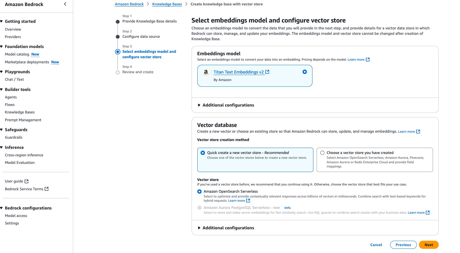
- On the Select embeddings model and configure vector store page, provide the following information:
- In the Embeddings model section, choose your embeddings model, which is used for embedding the chunks.
- In the Vector database section, create a new vector store or use an existing one where the embeddings will be stored for retrieval.
- Choose Next.
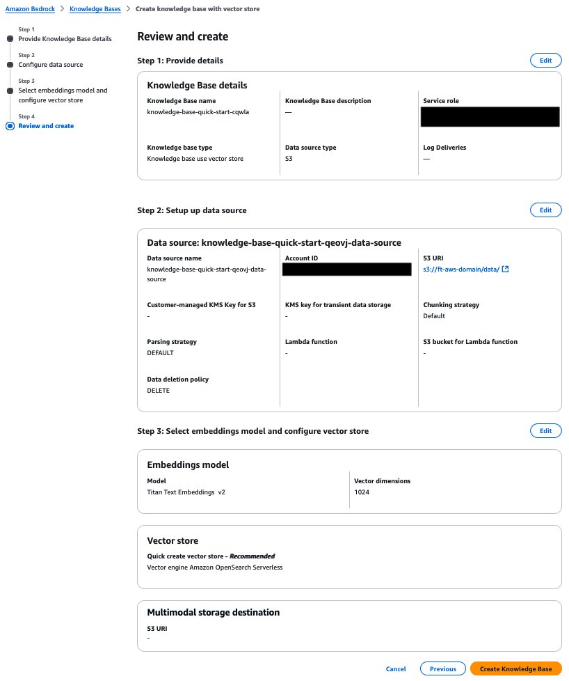
- On the Review and create page, review the settings and choose Create Knowledge Base.
Fine-tune an Amazon Nova model using the Amazon Bedrock API
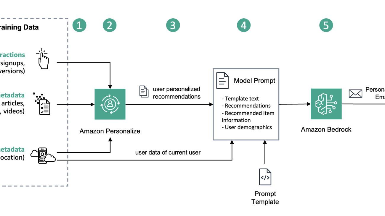
In this section, we provide detailed walkthroughs on fine-tuning and hosting customized Amazon Nova models using Amazon Bedrock. The following diagram illustrates the solution architecture.

Create a fine-tuning job
Fine-tuning Amazon Nova models through the Amazon Bedrock API is a streamlined process:
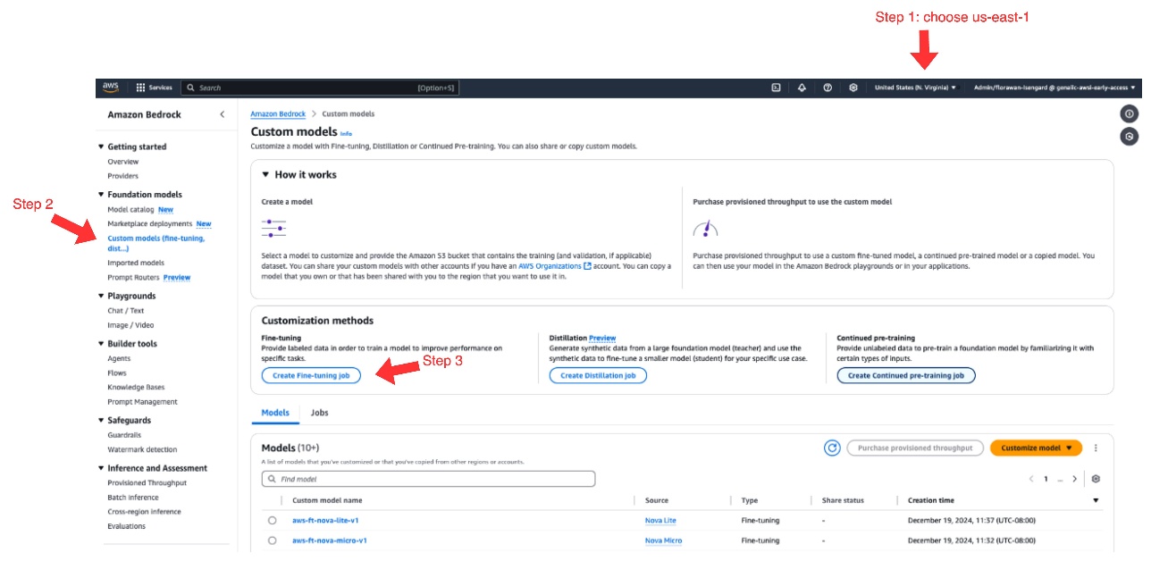
- On the Amazon Bedrock console, choose us-east-1 as your AWS Region.
At the time of writing, Amazon Nova model fine-tuning is exclusively available in us-east-1.
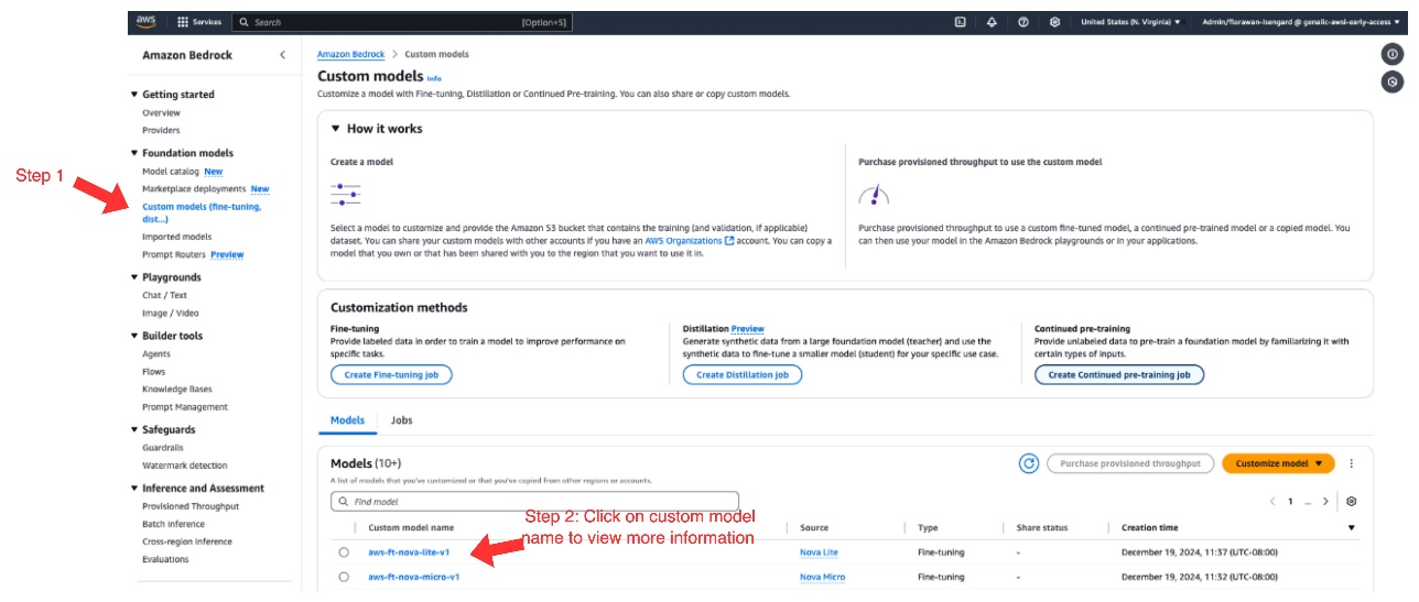
- Choose Custom models under Foundation models in the navigation pane.
- Under Customization methods, choose Create Fine-tuning job.
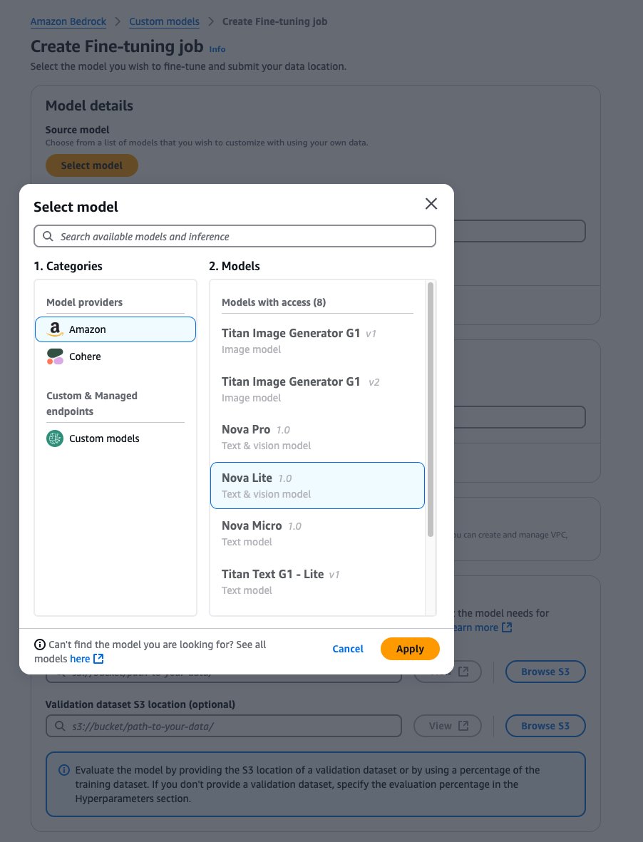
- For Source model, choose Select model.
- Choose Amazon as the provider and the Amazon Nova model of your choice.
- Choose Apply.
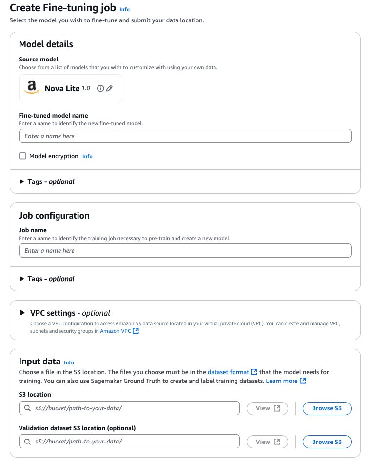
- For Fine-tuned model name, enter a unique name for the fine-tuned model.
- For Job name, enter a name for the fine-tuning job.
- Under Input data, enter the location of the source S3 bucket (training data) and target S3 bucket (model outputs and training metrics), and optionally the location of your validation dataset.
Configure hyperparameters
For Amazon Nova models, the following hyperparameters can be customized:
| Parameter |
Range/Constraints |
| Epochs |
1–5 |
| Batch Size |
Fixed at 1 |
| Learning Rate |
0.000001–0.0001 |
| Learning Rate Warmup Steps |
0–100 |
Prepare the dataset for compatibility with Amazon Nova models
Similar to other LLMs, Amazon Nova requires prompt-completion pairs, also known as question and answer (Q&A) pairs, for supervised fine-tuning (SFT). This dataset should contain the ideal outputs you want the language model to produce for specific tasks or prompts. Refer to Guidelines for preparing your data for Amazon Nova on best practices and example formats when preparing datasets for fine-tuning Amazon Nova models.
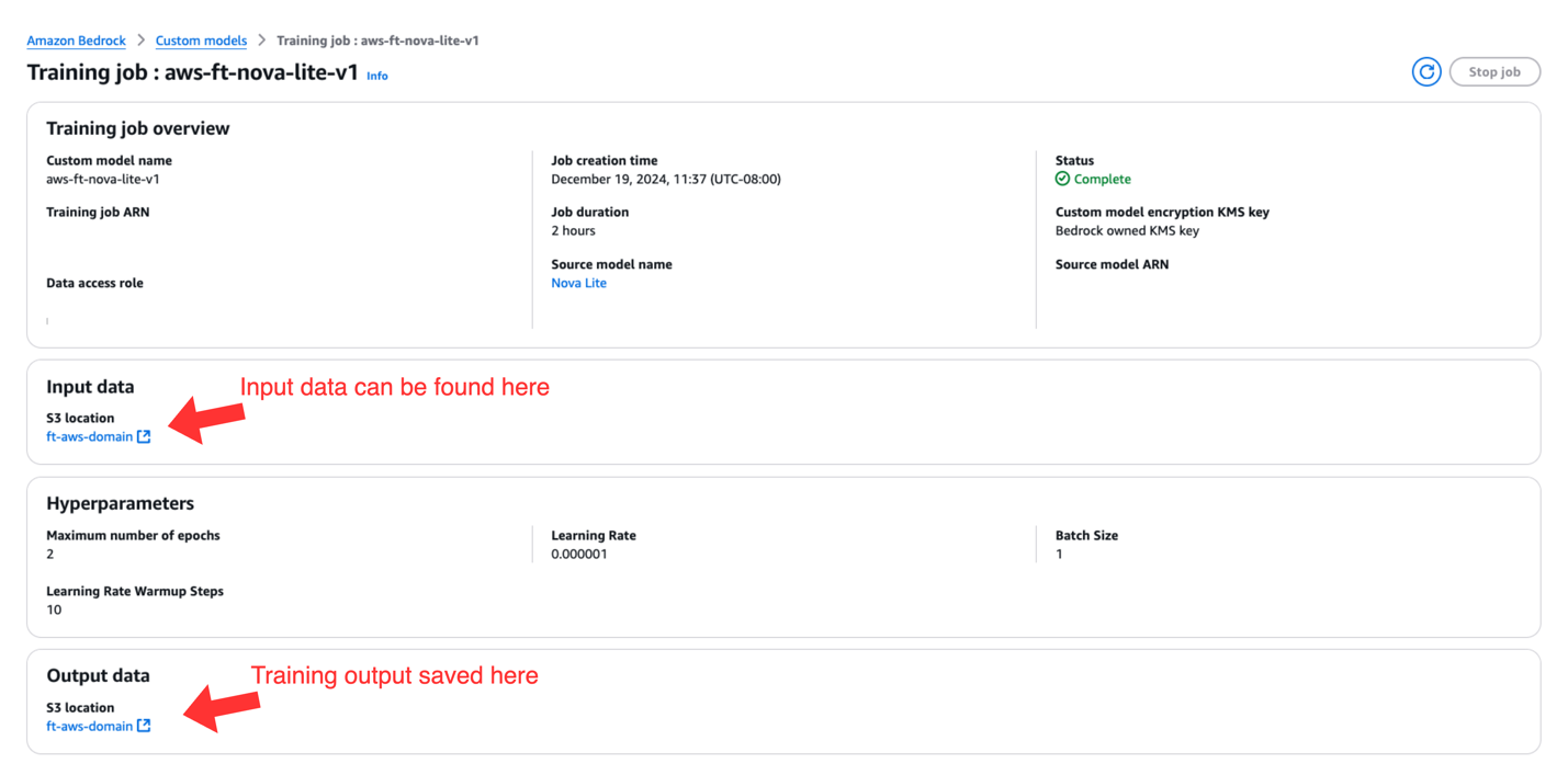
Examine fine-tuning job status and training artifacts
After you create your fine-tuning job, choose Custom models under Foundation models in the navigation pane. You will find the current fine-tuning job listed under Jobs. You can use this page to monitor your fine-tuning job status.
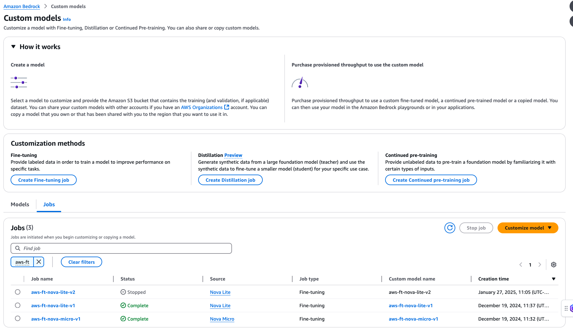
When your fine-tuning job status changes to Complete, you can choose the job name and navigate to the Training job overview page. You will find the following information:
- Training job specifications
- Amazon S3 location for input data used for fine-tuning
- Hyperparameters used during fine-tuning
- Amazon S3 location for training output
Host the fine-tuned model with provisioned throughput
After your fine-tuning job completes successfully, you can access your customized model through the following steps:
- On the Amazon Bedrock console, choose Custom models under Foundation models in the navigation pane.
- Under Models, choose your custom model.
The model details page shows the following information:
- Fine-tuned model details
- Amazon S3 location for input data used for fine-tuning
- Hyperparameters used during fine-tuning
- Amazon S3 location for training output
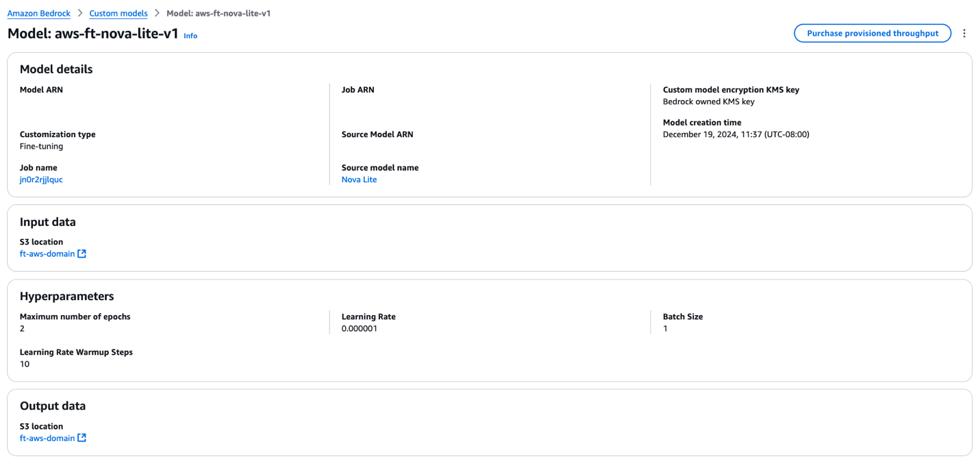
- To make your fine-tuned model available for inference, choose Purchase provisioned throughput.
- Choose a commitment term (no commitment, 1 month, or 6 months) and review the associated cost for hosting the fine-tuned models.
After the customized model is hosted through provisioned throughput, a model ID will be assigned and can be used for inference.
The aforementioned fine-tuning and inference steps can also be done programmatically. For more information, refer to the following GitHub repo, which contains sample code.
Evaluation framework and results
In this section, we first introduce our multi-LLM-judge evaluation framework, which is set up to mitigate an individual LLM judge’s bias. We then compare RAG vs. fine-tuning results in terms of response quality as well as latency and token implications.
Multiple LLMs as judges to mitigate bias
The following diagram illustrates our workflow using multiple LLMs as judges.
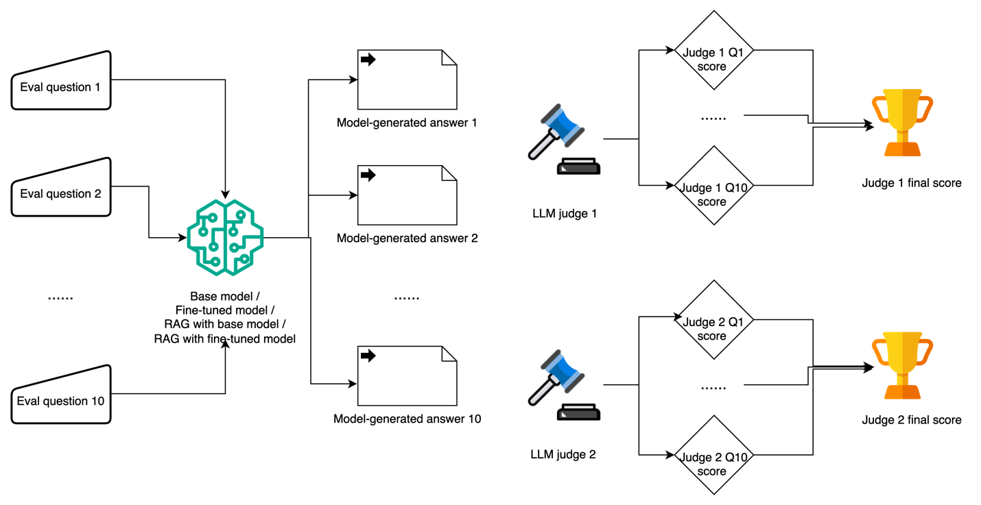
Using LLMs as judges has become an increasingly popular approach to evaluate tasks that are challenging to assess through traditional methods or human evaluation. For our evaluation framework, we constructed 10 domain-specific test questions covering key aspects of AWS services and features, designed to test both factual accuracy and depth of understanding. Each model-generated response was evaluated using a standardized scoring system on a scale of 0–10, where 0–3 indicates incorrect or misleading information, 4–6 represents partially correct but incomplete answers, 7–8 signifies mostly correct with minor inaccuracies, and 9–10 denotes completely accurate with comprehensive explanation.
We use the following LLM judge evaluation prompt:
{
    "system_prompt": "You are a helpful assistant.",
    "prompt_template": "[Instruction] Please act as an impartial judge and evaluate the quality of the response provided by an AI assistant to the user question displayed below. Your evaluation should consider factors such as the helpfulness, relevance, accuracy, depth, creativity, and level of detail of the response. Begin your evaluation by providing a short explanation. Be as objective as possible. After providing your explanation, you must rate the response on a scale of 1 to 10 by strictly following this format: "[[rating]]", for example: "Rating: [[5]]".nn[Question]n{question}nn[The Start of Assistant's Answer]n{answer}n[The End of Assistant's Answer]",
    "description": "Prompt for general questions",
    "category": "general",
    "output_format": "[[rating]]"
}
We use the following sample evaluation question and ground truth:
{
    "question_id": 9161,
    "category": "AWS",
    "turns": [
        " "What specific details are collected and sent to AWS when anonymous operational metrics are enabled for an Amazon EFS file system?",
        "What's required for a successful AWS CloudFormation launch?"
    ],
    "reference": [
        "When anonymous operational metrics are enabled for an Amazon EFS file system, the following specific details are collected and sent to AWS: Solution ID, Unique ID, Timestamp, Backup ID, Backup Start Time, Backup Stop Time, Backup Window, Source EFS Size, Destination EFS Size, Instance Type, Retain, S3 Bucket Size, Source Burst Credit Balance, Source Burst Credit Balance Post Backup, Source Performance Mode, Destination Performance Mode, Number of Files, Number of Files Transferred, Total File Size, Total Transferred File Size, Region, Create Hard Links Start Time, Create Hard Links Stop Time, Remove Snapshot Start Time, Remove Snapshot Stop Time, Rsync Delete Start Time, Rsync Delete Stop Time.",
        "For a successful AWS CloudFormation launch, you need to sign in to the AWS Management Console, choose the correct AWS Region, use the button to launch the template, verify the correct template URL, assign a name to your solution stack, review and modify the parameters as necessary, review and confirm the settings, check the boxes acknowledging that the template creates AWS Identity and Access Management resources and may require an AWS CloudFormation capability, and choose Create stack to deploy the stack. You should receive a CREATE_COMPLETE status in approximately 15 minutes."
    ]
}
To mitigate potential intrinsic biases among different LLM judges, we adopted two LLM judges to evaluate the model-generated responses: Anthropic’s Claude Sonnet 3.5 and Meta’s Llama 3.1 70B. Each judge was provided with the original test question, the model-generated response, and specific scoring criteria focusing on factual accuracy, completeness, relevance, and clarity. Overall, we observed a high level of rank correlation among LLM judges in assessing different approaches, with consistent evaluation patterns across all test cases.
Response quality comparison
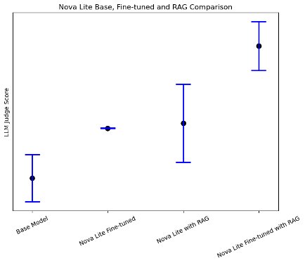
Both fine-tuning and RAG significantly improve the quality of generated responses on AWS-specific questions over the base model. Using Amazon Nova Lite as the base model, we observed that both fine-tuning and RAG improved the average LLM judge score on response quality by 30%, whereas combining fine-tuning with RAG enhanced the response quality by a total of 83%, as shown in the following figure.
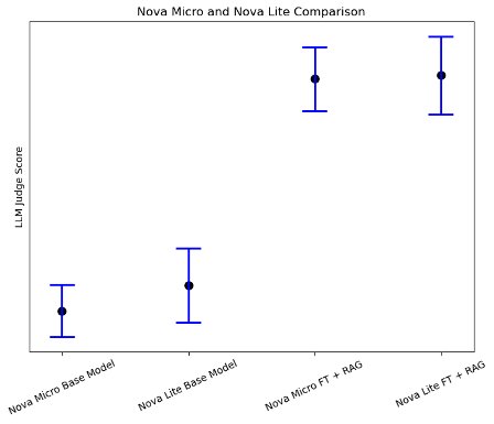
Notably, our evaluation revealed an interesting finding (as shown in the following figure): when combining fine-tuning and RAG approaches, smaller models like Amazon Nova Micro showed significant performance improvements in domain-specific tasks, nearly matching the performance of bigger models. This suggests that for specialized use cases with well-defined scope, using smaller models with both fine-tuning and RAG could be a more cost-effective solution compared to deploying larger models.
Latency and token implications
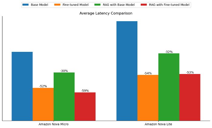
In addition to enhancing the response quality, both fine-tuning and RAG help reduce the response generation latency compared to the base model. For both Amazon Nova Micro and Amazon Nova Lite, fine-tuning reduced the base model latency by approximately 50%, whereas RAG reduced it by about 30%, as shown in the following figure.
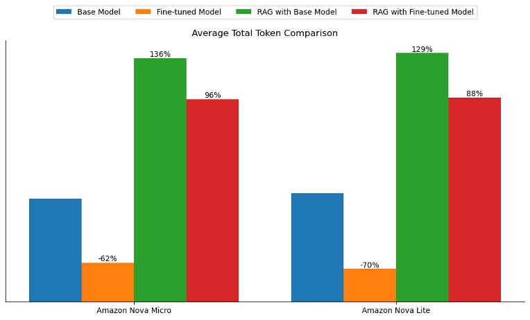
Fine-tuning also presented the unique advantage of improving the tone and style of the generated answers to align more closely with the training data. In our experiments, the average total tokens (input and output tokens) dropped by more than 60% with both fine-tuned models. However, the average total tokens more than doubled with the RAG approach due to passing of context, as shown in the following figure. This finding suggests that for latency-sensitive use cases or when the objective is to align the model’s responses to a specific tone, style, or brand voice, model customization might offer more business value.
Conclusion
In this post, we compared model customization (fine-tuning) and RAG for domain-specific tasks with Amazon Nova. We first provided a detailed walkthrough on how to fine-tune, host, and conduct inference with customized Amazon Nova through the Amazon Bedrock API. We then adopted an LLM-as-a-judge approach to evaluate response quality from different approaches. In addition, we examined the latency and token implications of different setups.
Both fine-tuning and RAG improved the model performance. Depending on the task and evaluation criteria, model customization showed similar, or sometimes better, performance compared to RAG. Model customization can also be helpful to improve the style and tone of a generated answer. In this experiment, the customized model’s response follows the succinct answer style of the given training data, which resulted in lower latency compared to the baseline counterpart. Additionally, model customization can also be used for many use cases where RAG isn’t as straightforward to be used, such as tool calling, sentiment analysis, entity extraction, and more. Overall, we recommend combining model customization and RAG for question answering or similar tasks to maximize performance.
For more information on Amazon Bedrock and the latest Amazon Nova models, refer to the Amazon Bedrock User Guide and Amazon Nova User Guide. The AWS Generative AI Innovation Center has a group of AWS science and strategy experts with comprehensive expertise spanning the generative AI journey, helping customers prioritize use cases, build a roadmap, and move solutions into production. Check out the Generative AI Innovation Center for our latest work and customer success stories.
About the Authors
 Mengdie (Flora) Wang is a Data Scientist at AWS Generative AI Innovation Center, where she works with customers to architect and implement scalable Generative AI solutions that address their unique business challenges. She specializes in model customization techniques and agent-based AI systems, helping organizations harness the full potential of generative AI technology. Prior to AWS, Flora earned her Master’s degree in Computer Science from the University of Minnesota, where she developed her expertise in machine learning and artificial intelligence.
 Sungmin Hong is a Senior Applied Scientist at Amazon Generative AI Innovation Center where he helps expedite the variety of use cases of AWS customers. Before joining Amazon, Sungmin was a postdoctoral research fellow at Harvard Medical School. He holds Ph.D. in Computer Science from New York University. Outside of work, he prides himself on keeping his indoor plants alive for 3+ years.
 Jae Oh Woo is a Senior Applied Scientist at the AWS Generative AI Innovation Center, where he specializes in developing custom solutions and model customization for a diverse range of use cases. He has a strong passion for interdisciplinary research that connects theoretical foundations with practical applications in the rapidly evolving field of generative AI. Prior to joining Amazon, Jae Oh was a Simons Postdoctoral Fellow at the University of Texas at Austin, where he conducted research across the Mathematics and Electrical and Computer Engineering departments. He holds a Ph.D. in Applied Mathematics from Yale University.
 Rahul Ghosh is an Applied Scientist at Amazon’s Generative AI Innovation Center, where he works with AWS customers across different verticals to expedite their use of Generative AI. Rahul holds a Ph.D. in Computer Science from the University of Minnesota.
 Baishali Chaudhury is an Applied Scientist at the Generative AI Innovation Center at AWS,
where she focuses on advancing Generative AI solutions for real-world applications. She has a
strong background in computer vision, machine learning, and AI for healthcare. Baishali holds a PhD in Computer Science from University of South Florida and PostDoc from Moffitt Cancer Centre.
 Anila Joshi has more than a decade of experience building AI solutions. As a AWSI Geo Leader at AWS Generative AI Innovation Center, Anila pioneers innovative applications of AI that push the boundaries of possibility and accelerate the adoption of AWS services with customers by helping customers ideate, identify, and implement secure generative AI solutions.
Read More


 Anoop Saha is a Sr GTM Specialist at Amazon Web Services (AWS) focusing on generative AI model training and inference. He partners with top frontier model builders, strategic customers, and AWS service teams to enable distributed training and inference at scale on AWS and lead joint GTM motions. Before AWS, Anoop held several leadership roles at startups and large corporations, primarily focusing on silicon and system architecture of AI infrastructure.
 Trevor Harvey is a Principal Specialist in generative AI at Amazon Web Services (AWS) and an AWS Certified Solutions Architect – Professional. Trevor works with customers to design and implement machine learning solutions and leads go-to-market strategies for generative AI services.
 Aman Shanbhag is a Specialist Solutions Architect on the ML Frameworks team at Amazon Web Services (AWS), where he helps customers and partners with deploying ML training and inference solutions at scale. Before joining AWS, Aman graduated from Rice University with degrees in computer science, mathematics, and entrepreneurship.
 We’re teaming up with Range Media Partners to announce AI on Screen, a new short film program.
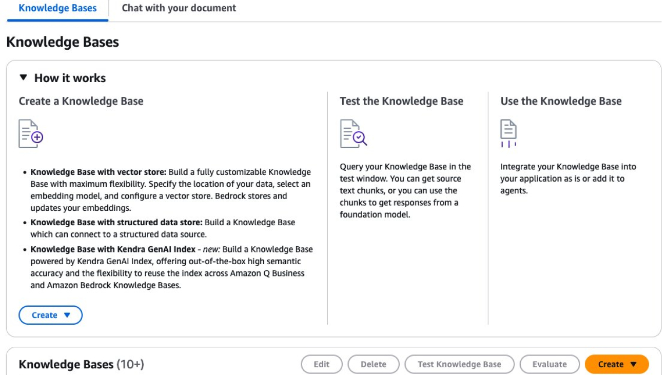

 Anna Grüebler Clark is a Specialist Solutions Architect at AWS focusing on in Artificial Intelligence. She has more than 16 years experience helping customers develop and deploy machine learning applications. Her passion is taking new technologies and putting them in the hands of everyone, and solving difficult problems leveraging the advantages of using traditional and generative AI in the cloud.


 Balu Mathew is a Senior Solutions Architect at AWS, based in Raleigh, NC. He collaborates with Global Financial Services customers to design and implement secure, scalable and resilient solutions on AWS. With deep expertise in security, machine learning, and the financial services industry, he helps organizations build, protect, and scale large-scale distributed systems efficiently. Outside of work, he enjoys spending time with his kids and exploring the mountains and the outdoors.


 Deepesh Dhapola is a Senior Solutions Architect at AWS India, specializing in helping financial services and fintech clients optimize and scale their applications on the AWS Cloud. With a strong focus on trending AI technologies, including generative AI, AI agents, and the Model Context Protocol (MCP), Deepesh leverages his expertise in machine learning to design innovative, scalable, and secure solutions. Passionate about the transformative potential of AI, he actively explores cutting-edge advancements to drive efficiency and innovation for AWS customers. Outside of work, Deepesh enjoys spending quality time with his family and experimenting with diverse culinary creations.
 Andre Boaventura is a Principal AI/ML Solutions Architect at AWS, specializing in generative AI and scalable machine learning solutions. With over 25 years in the high-tech software industry, he has deep expertise in designing and deploying AI applications using AWS services such as Amazon Bedrock, Amazon SageMaker, and Amazon Q. Andre works closely with global system integrators (GSIs) and customers across industries to architect and implement cutting-edge AI/ML solutions to drive business value.
 Preston Tuggle is a Sr. Specialist Solutions Architect with the Third-Party Model Provider team at AWS. He focuses on working with model providers across Amazon Bedrock and Amazon SageMaker, helping them accelerate their go-to-market strategies through technical scaling initiatives and customer engagement
 Shane Rai is a Principal GenAI Specialist with the AWS World Wide Specialist Organization (WWSO). He works with customers across industries to solve their most pressing and innovative business needs using AWS’s breadth of cloud-based AI/ML services, including model offerings from top-tier foundation model providers.
 Ankit Agarwal is a Senior Technical Product Manager at Amazon Bedrock, where he operates at the intersection of customer needs and foundation model providers. He leads initiatives to onboard cutting-edge models onto Amazon Bedrock Serverless and drives the development of core features that enhance the platform’s capabilities.
 Niithiyn Vijeaswaran is a Generative AI Specialist Solutions Architect with the Third-Party Model Science team at AWS. His area of focus is AWS AI accelerators (AWS Neuron). He holds a Bachelor’s in Computer Science and Bioinformatics.
 Aris Tsakpinis is a Specialist Solutions Architect for Generative AI focusing on open source models on Amazon Bedrock and the broader generative AI open source ecosystem. Alongside his professional role, he is pursuing a PhD in Machine Learning Engineering at the University of Regensburg, where his research focuses on applied natural language processing in scientific domains.