Monthly Archives: April 2025

Modern large language models (LLMs) excel in language processing but are limited by their static training data. However, as industries require more adaptive, decision-making AI, integrating tools and external APIs has become essential. This has led to the evolution and rapid rise of agentic workflows, where AI systems autonomously plan, execute, and refine tasks. Accurate tool use is foundational for enhancing the decision-making and operational efficiency of these autonomous agents and building successful and complex agentic workflows.

In this post, we dissect the technical mechanisms of tool calling using Amazon Nova models through Amazon Bedrock, alongside methods for model customization to refine tool calling precision.

Expanding LLM capabilities with tool use

LLMs excel at natural language tasks but become significantly more powerful with tool integration, such as APIs and computational frameworks. Tools enable LLMs to access real-time data, perform domain-specific computations, and retrieve precise information, enhancing their reliability and versatility. For example, integrating a weather API allows for accurate, real-time forecasts, or a Wikipedia API provides up-to-date information for complex queries. In scientific contexts, tools like calculators or symbolic engines address numerical inaccuracies in LLMs. These integrations transform LLMs into robust, domain-aware systems capable of handling dynamic, specialized tasks with real-world utility.

Amazon Nova models and Amazon Bedrock

Amazon Nova models, unveiled at AWS re:Invent in December 2024, are optimized to deliver exceptional price-performance value, offering state-of-the-art performance on key text-understanding benchmarks at low cost. The series comprises three variants: Micro (text-only, ultra-efficient for edge use), Lite (multimodal, balanced for versatility), and Pro (multimodal, high-performance for complex tasks).

Amazon Nova models can be used for variety of tasks, from generation to developing agentic workflows. As such, these models have the capability to interface with external tools or services and use them through tool calling. This can be achieved through the Amazon Bedrock console (see Getting started with Amazon Nova in the Amazon Bedrock console) and APIs such as Converse and Invoke.

In addition to using the pre-trained models, developers have the option to fine-tune these models with multimodal data (Pro and Lite) or text data (Pro, Lite, and Micro), providing the flexibility to achieve desired accuracy, latency, and cost. Developers can also run self-service custom fine-tuning and distillation of larger models to smaller ones using the Amazon Bedrock console and APIs.

Solution overview

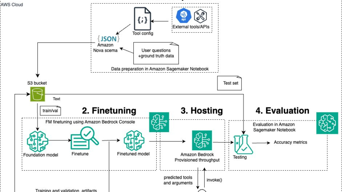
The following diagram illustrates the solution architecture.

For this post, we first prepared a custom dataset for tool usage. We used the test set to evaluate Amazon Nova models through Amazon Bedrock using the Converse and Invoke APIs. We then fine-tuned Amazon Nova Micro and Amazon Nova Lite models through Amazon Bedrock with our fine-tuning dataset. After the fine-tuning process was complete, we evaluated these customized models through provisioned throughput. In the following sections, we go through these steps in more detail.

Tools

Tool usage in LLMs involves two critical operations: tool selection and argument extraction or generation. For instance, consider a tool designed to retrieve weather information for a specific location. When presented with a query such as “What’s the weather in Alexandria, VA?”, the LLM evaluates its repertoire of tools to determine whether an appropriate tool is available. Upon identifying a suitable tool, the model selects it and extracts the required arguments—here, “Alexandria” and “VA” as structured data types (for example, strings)—to construct the tool call.

Each tool is rigorously defined with a formal specification that outlines its intended functionality, the mandatory or optional arguments, and the associated data types. Such precise definitions, known as tool config, make sure that tool calls are executed correctly and that argument parsing aligns with the tool’s operational requirements. Following this requirement, the dataset used for this example defines eight tools with their arguments and configures them in a structured JSON format. We define the following eight tools (we use seven of them for fine-tuning and hold out the weather_api_call tool during testing in order to evaluate the accuracy on unseen tool use):

• weather_api_call – Custom tool for getting weather information
• stat_pull – Custom tool for identifying stats
• text_to_sql – Custom text-to-SQL tool
• terminal – Tool for executing scripts in a terminal
• wikipidea – Wikipedia API tool to search through Wikipedia pages
• duckduckgo_results_json – Internet search tool that executes a DuckDuckGo search
• youtube_search – YouTube API search tool that searches video listings
• pubmed_search – PubMed search tool that searches PubMed abstracts

The following code is an example of what a tool configuration for terminal might look like:

{'toolSpec': {'name': 'terminal',
'description': 'Run shell commands on this MacOS machine ',
'inputSchema': {'json': {'type': 'object',
'properties': {'commands': {'type': 'string',
'description': 'List of shell commands to run. Deserialized using json.loads'}},
'required': ['commands']}}}},

Dataset

The dataset is a synthetic tool calling dataset created with assistance from a foundation model (FM) from Amazon Bedrock and manually validated and adjusted. This dataset was created for our set of eight tools as discussed in the previous section, with the goal of creating a diverse set of questions and tool invocations that allow another model to learn from these examples and generalize to unseen tool invocations.

Each entry in the dataset is structured as a JSON object with key-value pairs that define the question (a natural language user query for the model), the ground truth tool required to answer the user query, its arguments (dictionary containing the parameters required to execute the tool), and additional constraints like order_matters: boolean, indicating if argument order is critical, and arg_pattern: optional, a regular expression (regex) for argument validation or formatting. Later in this post, we use these ground truth labels to supervise the training of pre-trained Amazon Nova models, adapting them for tool use. This process, known as supervised fine-tuning, will be explored in detail in the following sections.

The size of the training set is 560 questions and the test set is 120 questions. The test set consists of 15 questions per tool category, totaling 120 questions. The following are some examples from the dataset:

{
"question": "Explain the process of photosynthesis",
"answer": "wikipedia",
"args": {'query': 'process of photosynthesis'
},
"order_matters":False,
"arg_pattern":None
}
{
"question": "Display system date and time",
"answer": "terminal",
"args": {'commands': ['date'
]
},
"order_matters":True,
"arg_pattern":None
}
{
"question": "Upgrade the requests library using pip",
"answer": "terminal",
"args": {'commands': ['pip install --upgrade requests'
]
},
"order_matters":True,
"arg_pattern": [r'pip(3?) install --upgrade requests'
]
}

Prepare the dataset for Amazon Nova

To use this dataset with Amazon Nova models, we need to additionally format the data based on a particular chat template. Native tool calling has a translation layer that formats the inputs to the appropriate format before passing the model. Here, we employ a DIY tool use approach with a custom prompt template. Specifically, we need to add the system prompt, the user message embedded with the tool config, and the ground truth labels as the assistant message. The following is a training example formatted for Amazon Nova. Due to space constraints, we only show the toolspec for one tool.

{"system": [{"text": "You are a bot that can handle different requests
with tools."}],
"messages": [{"role": "user",
"content": [{"text": "Given the following functions within <tools>,
please respond with a JSON for a function call with its proper arguments
that best answers the given prompt.

Respond in the format
{"name": function name,"parameters": dictionary of argument name and
its value}.
Do not use variables. Donot give any explanations.

ONLY output the resulting
JSON structure and nothing else.

Donot use the word 'json' anywhere in the
result.
<tools>
    {"tools": [{"toolSpec":{"name":"youtube_search",
    "description": " search for youtube videos associated with a person.
    the input to this tool should be a comma separated list, the first part
    contains a person name and the second a number that is the maximum number
    of video results to return aka num_results. the second part is optional", 
    "inputSchema":
    {"json":{"type":"object","properties": {"query":
    {"type": "string",
     "description": "youtube search query to look up"}},
    "required": ["query"]}}}},]}
</tools>
Generate answer for the following question.
<question>
List any products that have received consistently negative reviews
</question>"}]},
{"role": "assistant", "content": [{"text": "{'name':text_to_sql,'parameters':
{'table': 'product_reviews','condition':
'GROUP BY product_id HAVING AVG(rating) < 2'}}"}]}],
"schemaVersion": "tooluse-dataset-2024"}

Upload dataset to Amazon S3

This step is needed later for the fine-tuning for Amazon Bedrock to access the training data. You can upload your dataset either through the Amazon Simple Storage Service (Amazon S3) console or through code.

Tool calling with base models through the Amazon Bedrock API

Now that we have created the tool use dataset and formatted it as required, let’s use it to test out the Amazon Nova models. As mentioned previously, we can use both the Converse and Invoke APIs for tool use in Amazon Bedrock. The Converse API enables dynamic, context-aware conversations, allowing models to engage in multi-turn dialogues, and the Invoke API allows the user to call and interact with the underlying models within Amazon Bedrock.

To use the Converse API, you simply send the messages, system prompt (if any), and the tool config directly in the Converse API. See the following example code:

response = bedrock_runtime.converse(
modelId=model_id,
messages=messages,
system=system_prompt,
toolConfig=tool_config,
)

To parse the tool and arguments from the LLM response, you can use the following example code:

for content_block in response['output']['message']["content"]:

if "toolUse" in content_block:
out_tool_name=content_block['toolUse']['name']
out_tool_inputs_dict=content_block['toolUse']['input']
print(out_tool_name,out_tool_inputs_dict.keys())

For the question: “Hey, what's the temperature in Paris right now?”, you get the following output:

weather_api_call dict_keys(['country', 'city'])

To execute tool use through the Invoke API, first you need to prepare the request body with the user question as well as the tool config that was prepared before. The following code snippet shows how to convert the tool config JSON to string format, which can be used in the message body:

# Convert tools configuration to JSON string
formatted_tool_config = json.dumps(tool_config, indent=2)
prompt = prompt_template.replace("{question}", question)
prompt = prompt.replace("{tool_config}", formatted_tool_config)
# message template
messages = [{"role": "user", "content": [{"text": prompt}]}]
# Prepare request body
model_kwargs = {"system":system_prompt, "messages": messages, "inferenceConfig": inferenceConfig,} body = json.dumps(model_kwargs)
response = bedrock_runtime.invoke_model(
body=body,
modelId=model_id,
accept=accept,
contentType=contentType
)

Using either of the two APIs, you can test and benchmark the base Amazon Nova models with the tool use dataset. In the next sections, we show how you can customize these base models specifically for the tool use domain.

Supervised fine-tuning using the Amazon Bedrock console

Amazon Bedrock offers three different customization techniques: supervised fine-tuning, model distillation, and continued pre-training. At the time of writing, the first two methods are available for customizing Amazon Nova models. Supervised fine-tuning is a popular method in transfer learning, where a pre-trained model is adapted to a specific task or domain by training it further on a smaller, task-specific dataset. The process uses the representations learned during pre-training on large datasets to improve performance in the new domain. During fine-tuning, the model’s parameters (either all or selected layers) are updated using backpropagation to minimize the loss.

In this post, we use the labeled datasets that we created and formatted previously to run supervised fine-tuning to adapt Amazon Nova models for the tool use domain.

Create a fine-tuning job

Complete the following steps to create a fine-tuning job:

1. Open the Amazon Bedrock console.
2. Choose us-east-1 as the AWS Region.
3. Under Foundation models in the navigation pane, choose Custom models.
4. Choose Create Fine-tuning job under Customization methods. 

At the time of writing, Amazon Nova model fine-tuning is exclusively available in the us-east-1 Region.

5. Choose Select model and choose Amazon as the model provider.
6. Choose your model (for this post, Amazon Nova Micro) and choose Apply.

7. For Fine-tuned model name, enter a unique name.
8. For Job name¸ enter a name for the fine-tuning job.
9. In the Input data section, enter following details:
   • For S3 location, enter the source S3 bucket containing the training data.
   • For Validation dataset location, optionally enter the S3 bucket containing a validation dataset.

10. In the Hyperparameters section, you can customize the following hyperparameters:
    • For Epochs¸ enter a value between 1–5.
    • For Batch size, the value is fixed at 1.
    • For Learning rate multiplier, enter a value between 0.000001–0.0001
    • For Learning rate warmup steps, enter a value between 0–100.

We recommend starting with the default parameter values and then changing the settings iteratively. It’s a good practice to change only one or a couple of parameters at a time, in order to isolate the parameter effects. Remember, hyperparameter tuning is model and use case specific.

11. In the Output data section, enter the target S3 bucket for model outputs and training metrics.
12. Choose Create fine-tuning job.

Run the fine-tuning job

After you start the fine-tuning job, you will be able to see your job under Jobs and the status as Training. When it finishes, the status changes to Complete.

You can now go to the training job and optionally access the training-related artifacts that are saved in the output folder.

You can find both training and validation (we highly recommend using a validation set) artifacts here.

You can use the training and validation artifacts to assess your fine-tuning job through loss curves (as shown in the following figure), which track training loss (orange) and validation loss (blue) over time. A steady decline in both indicates effective learning and good generalization. A small gap between them suggests minimal overfitting, whereas a rising validation loss with decreasing training loss signals overfitting. If both losses remain high, it indicates underfitting. Monitoring these curves helps you quickly diagnose model performance and adjust training strategies for optimal results.

Host the fine-tuned model and run inference

Now that you have completed the fine-tuning, you can host the model and use it for inference. Follow these steps:

1. On the Amazon Bedrock console, under Foundation models in the navigation pane, choose Custom models
2. On the Models tab, choose the model you fine-tuned.

3. Choose Purchase provisioned throughput.

4. Specify a commitment term (no commitment, 1 month, 6 months) and review the associated cost for hosting the fine-tuned models.

After the customized model is hosted through provisioned throughput, a model ID will be assigned, which will be used for inference. For inference with models hosted with provisioned throughput, we have to use the Invoke API in the same way we described previously in this post—simply replace the model ID with the customized model ID.

The aforementioned fine-tuning and inference steps can also be done programmatically. Refer to the following GitHub repo for more detail.

Evaluation framework

Evaluating fine-tuned tool calling LLMs requires a comprehensive approach to assess their performance across various dimensions. The primary metric to evaluate tool calling is accuracy, including both tool selection and argument generation accuracy. This measures how effectively the model selects the correct tool and generates valid arguments. Latency and token usage (input and output tokens) are two other important metrics.

Tool call accuracy evaluates if the tool predicted by the LLM matches the ground truth tool for each question; a score of 1 is given if they match and 0 when they don’t. After processing the questions, we can use the following equation: Tool Call Accuracy=∑(Correct Tool Calls)/(Total number of test questions).

Argument call accuracy assesses whether the arguments provided to the tools are correct, based on either exact matches or regex pattern matching. For each tool call, the model’s predicted arguments are extracted. It uses the following argument matching methods:

• Regex matching – If the ground truth includes regex patterns, the predicted arguments are matched against these patterns. A successful match increases the score.
• Inclusive string matching – If no regex pattern is provided, the predicted argument is compared to the ground truth argument. Credit is given if the predicted argument contains the ground truth argument. This is to allow for arguments, like search terms, to not be penalized for adding additional specificity.

The score for each argument is normalized based on the number of arguments, allowing partial credit when multiple arguments are required. The cumulative correct argument scores are averaged across all questions: Argument Call Accuracy = ∑Correct Arguments/(Total Number of Questions).

Below we show some example questions and accuracy scores:

Example 1:

User question: Execute this run.py script with an argparse arg adding two gpus
GT tool: terminal   LLM output tool: terminal
Pred args:  ['python run.py —gpus 2']
Ground truth pattern: python(3?) run.py —gpus 2
Arg matching method: regex match
Arg matching score: 1.0

Example 2:

User question: Who had the most rushing touchdowns for the bengals in 2017 season?
GT tool: stat_pull   LLM output tool: stat_pull
Pred args:  ['NFL']
straight match
arg score 0.3333333333333333
Pred args:  ['2017']
Straight match
Arg score 0.6666666666666666
Pred args:  ['Cincinnati Bengals']
Straight match
Arg score 1.0

Results

We are now ready to visualize the results and compare the performance of base Amazon Nova models to their fine-tuned counterparts.

Base models

The following figures illustrate the performance comparison of the base Amazon Nova models.

The comparison reveals a clear trade-off between accuracy and latency, shaped by model size. Amazon Nova Pro, the largest model, delivers the highest accuracy in both tool call and argument call tasks, reflecting its advanced computational capabilities. However, this comes with increased latency.

In contrast, Amazon Nova Micro, the smallest model, achieves the lowest latency, which ideal for fast, resource-constrained environments, though it sacrifices some accuracy compared to its larger counterparts.

Fine-tuned models vs. base models

The following figure visualizes accuracy improvement after fine-tuning.

The comparative analysis of the Amazon Nova model variants reveals substantial performance improvements through fine-tuning, with the most significant gains observed in the smaller Amazon Nova Micro model. The fine-tuned Amazon Nova model showed remarkable growth in tool call accuracy, increasing from 75.8% to 95%, which is a 25.38% improvement. Similarly, its argument call accuracy rose from 77.8% to 87.7%, reflecting a 12.74% increase.

In contrast, the fine-tuned Amazon Nova Lite model exhibited more modest gains, with tool call accuracy improving from 90.8% to 96.66%—a 6.46% increase—and argument call accuracy rising from 85% to 89.9%, marking a 5.76% improvement. Both fine-tuned models surpassed the accuracy achieved by the Amazon Nova Pro base model.

These results highlight that fine-tuning can significantly enhance the performance of lightweight models, making them strong contenders for applications where both accuracy and latency are critical.

Conclusion

In this post, we demonstrated model customization (fine-tuning) for tool use with Amazon Nova. We first introduced a tool usage use case, and gave details about the dataset. We walked through the details of Amazon Nova specific data formatting and showed how to do tool calling through the Converse and Invoke APIs in Amazon Bedrock. After getting the baseline results from Amazon Nova models, we explained in detail the fine-tuning process, hosting fine-tuned models with provisioned throughput, and using the fine-tuned Amazon Nova models for inference. In addition, we touched upon getting insights from training and validation artifacts from a fine-tuning job in Amazon Bedrock.

Check out the detailed notebook for tool usage to learn more. For more information on Amazon Bedrock and the latest Amazon Nova models, refer to the Amazon Bedrock User Guide and Amazon Nova User Guide. The Generative AI Innovation Center has a group of AWS science and strategy experts with comprehensive expertise spanning the generative AI journey, helping customers prioritize use cases, build roadmaps, and move solutions into production. See Generative AI Innovation Center for our latest work and customer success stories.

About the Authors

Baishali Chaudhury is an Applied Scientist at the Generative AI Innovation Center at AWS, where she focuses on advancing Generative AI solutions for real-world applications. She has a strong background in computer vision, machine learning, and AI for healthcare. Baishali holds a PhD in Computer Science from University of South Florida and PostDoc from Moffitt Cancer Centre.

Isaac Privitera is a Principal Data Scientist with the AWS Generative AI Innovation Center, where he develops bespoke generative AI-based solutions to address customers’ business problems. His primary focus lies in building responsible AI systems, using techniques such as RAG, multi-agent systems, and model fine-tuning. When not immersed in the world of AI, Isaac can be found on the golf course, enjoying a football game, or hiking trails with his loyal canine companion, Barry.

Mengdie (Flora) Wang is a Data Scientist at AWS Generative AI Innovation Center, where she works with customers to architect and implement scalableGenerative AI solutions that address their unique business challenges. She specializes in model customization techniques and agent-based AI systems, helping organizations harness the full potential of generative AI technology. Prior to AWS, Flora earned her Master’s degree in Computer Science from the University of Minnesota, where she developed her expertise in machine learning and artificial intelligence.

Read More

AI agents are quickly becoming an integral part of customer workflows across industries by automating complex tasks, enhancing decision-making, and streamlining operations. However, the adoption of AI agents in production systems requires scalable evaluation pipelines. Robust agent evaluation enables you to gauge how well an agent is performing certain actions and gain key insights into them, enhancing AI agent safety, control, trust, transparency, and performance optimization.

Amazon Bedrock Agents uses the reasoning of foundation models (FMs) available on Amazon Bedrock, APIs, and data to break down user requests, gather relevant information, and efficiently complete tasks—freeing teams to focus on high-value work. You can enable generative AI applications to automate multistep tasks by seamlessly connecting with company systems, APIs, and data sources.

Ragas is an open source library for testing and evaluating large language model (LLM) applications across various LLM use cases, including Retrieval Augmented Generation (RAG). The framework enables quantitative measurement of the effectiveness of the RAG implementation. In this post, we use the Ragas library to evaluate the RAG capability of Amazon Bedrock Agents.

LLM-as-a-judge is an evaluation approach that uses LLMs to assess the quality of AI-generated outputs. This method employs an LLM to act as an impartial evaluator, to analyze and score outputs. In this post, we employ the LLM-as-a-judge technique to evaluate the text-to-SQL and chain-of-thought capabilities of Amazon Bedrock Agents.

Langfuse is an open source LLM engineering platform, which provides features such as traces, evals, prompt management, and metrics to debug and improve your LLM application.

In the post Accelerate analysis and discovery of cancer biomarkers with Amazon Bedrock Agents, we showcased research agents for cancer biomarker discovery for pharmaceutical companies. In this post, we extend the prior work and showcase Open Source Bedrock Agent Evaluation with the following capabilities:

• Evaluating Amazon Bedrock Agents on its capabilities (RAG, text-to-SQL, custom tool use) and overall chain-of-thought
• Comprehensive evaluation results and trace data sent to Langfuse with built-in visual dashboards
• Trace parsing and evaluations for various Amazon Bedrock Agents configuration options

First, we conduct evaluations on a variety of different Amazon Bedrock Agents. These include a sample RAG agent, a sample text-to-SQL agent, and pharmaceutical research agents that use multi-agent collaboration for cancer biomarker discovery. Then, for each agent, we showcase navigating the Langfuse dashboard to view traces and evaluation results.

Technical challenges

Today, AI agent developers generally face the following technical challenges:

• End-to-end agent evaluation – Although Amazon Bedrock provides built-in evaluation capabilities for LLM models and RAG retrieval, it lacks metrics specifically designed for Amazon Bedrock Agents. There is a need for evaluating the holistic agent goal, as well as individual agent trace steps for specific tasks and tool invocations. Support is also needed for both single and multi-agents, and both single and multi-turn datasets.
• Challenging experiment management – Amazon Bedrock Agents offers numerous configuration options, including LLM model selection, agent instructions, tool configurations, and multi-agent setups. However, conducting rapid experimentation with these parameters is technically challenging due to the lack of systematic ways to track, compare, and measure the impact of configuration changes across different agent versions. This makes it difficult to effectively optimize agent performance through iterative testing.

Solution overview

The following figure illustrates how Open Source Bedrock Agent Evaluation works on a high level. The framework runs an evaluation job that will invoke your own agent in Amazon Bedrock and evaluate its response.

The workflow consists of the following steps:

1. The user specifies the agent ID, alias, evaluation model, and dataset containing question and ground truth pairs.
2. The user executes the evaluation job, which will invoke the specified Amazon Bedrock agent.
3. The retrieved agent invocation traces are run through a custom parsing logic in the framework.
4. The framework conducts an evaluation based on the agent invocation results and the question type:
   1. Chain-of-thought – LLM-as-a-judge with Amazon Bedrock LLM calls (conducted for every evaluation run for different types of questions)
   2. RAG – Ragas evaluation library
   3. Text-to-SQL – LLM-as-a-judge with Amazon Bedrock LLM calls
5. Evaluation results and parsed traces are gathered and sent to Langfuse for evaluation insights.

Prerequisites

To deploy the sample RAG and text-to-SQL agents and follow along with evaluating them using Open Source Bedrock Agent Evaluation, follow the instructions in Deploying Sample Agents for Evaluation.

To bring your own agent to evaluate with this framework, refer to the following README and follow the detailed instructions to deploy the Open Source Bedrock Agent Evaluation framework.

Overview of evaluation metrics and input data

First, we create sample Amazon Bedrock agents to demonstrate the capabilities of Open Source Bedrock Agent Evaluation. The text-to-SQL agent uses the BirdSQL Mini-Dev dataset, and the RAG agent uses the Hugging Face rag-mini-wikpedia dataset.

Evaluation metrics

The Open Source Bedrock Agent Evaluation framework conducts evaluations on two broad types of metrics:

• Agent goal – Chain-of-thought (run on every question)
• Task accuracy – RAG, text-to-SQL (run only when the specific tool is used to answer question)

Agent goal metrics measure how well an agent identifies and achieves the goals of the user. There are two main types: reference-based evaluation and no reference evaluation. Examples can be found in Agent Goal accuracy as defined by Ragas:

• Reference-based evaluation – The user provides a reference that will be used as the ideal outcome. The metric is computed by comparing the reference with the goal achieved by the end of the workflow.
• Evaluation without reference – The metric evaluates the performance of the LLM in identifying and achieving the goals of the user without reference.

We will showcase evaluation without reference using chain-of-thought evaluation. We conduct evaluations by comparing the agent’s reasoning and the agent’s instruction. For this evaluation, we use some metrics from the evaluator prompts for Amazon Bedrock LLM-as-a-judge. In this framework, the chain-of-thought evaluations are run on every question that the agent is evaluated against.

Task accuracy metrics measure how well an agent calls the required tools to complete a given task. For the two task accuracy metrics, RAG and text-to-SQL, evaluations are conducted based on comparing the actual agent answer against the ground truth dataset that must be provided in the input dataset. The task accuracy metrics are only evaluated when the corresponding tool is used to answer the question.

The following is a breakdown of the key metrics used in each evaluation type included in the framework:

• RAG:
  • Faithfulness – How factually consistent a response is with the retrieved context
  • Answer relevancy – How directly and appropriately the original question is addressed
  • Context recall – How many of the relevant pieces of information were successfully retrieved
  • Semantic similarity – The assessment of the semantic resemblance between the generated answer and the ground truth
• Text-to-SQL:
  • SQL query semantic equivalence – The equivalence of response query with the reference query
  • Answer correctness – How well the generated answer correctly represents the query results and matches ground truth
• Chain-of-thought:
  • Helpfulness – How well the agent satisfies explicit and implicit expectations
  • Faithfulness – How well the agent sticks to available information and context
  • Instruction following – How well the agent respects all explicit directions

User-agent trajectories

The input dataset is in the form of trajectories, where each trajectory consists of one or more questions to be answered by the agent. The trajectories are meant to simulate how a user might interact with the agent. Each trajectory consists of a unique question_id, question_type, question, and ground_truth information. The following are examples of actual trajectories used to evaluate each type of agent in this post.

For more simple agent setups like the RAG and text-to-SQL sample agent, we created trajectories consisting of a single question, as shown in the following examples.

The following is an example of a RAG sample agent trajectory:

{
	"Trajectory0": [
		{
			"question_id": 0,
			"question_type": "RAG",
			"question": "Was Abraham Lincoln the sixteenth President of the United States?",
			"ground_truth": "yes"
		}
	]
}

The following is an example of a text-to-SQL sample agent trajectory:

{
	"Trajectory1": [
		{
			"question_id": 1,
			"question": "What is the highest eligible free rate for K-12 students in the schools in Alameda County?",
			"question_type": "TEXT2SQL",
			"ground_truth": {
				"ground_truth_sql_query": "SELECT `Free Meal Count (K-12)` / `Enrollment (K-12)` FROM frpm WHERE `County Name` = 'Alameda' ORDER BY (CAST(`Free Meal Count (K-12)` AS REAL) / `Enrollment (K-12)`) DESC LIMIT 1",
				"ground_truth_sql_context": "[{'table_name': 'frpm', 'columns': [('cdscode', 'varchar'), ('academic year', 'varchar'), ...",
				"ground_truth_query_result": "1.0",
				"ground_truth_answer": "The highest eligible free rate for K-12 students in schools in Alameda County is 1.0."
		}
	]
}

Pharmaceutical research agent use case example

In this section, we demonstrate how you can use the Open Source Bedrock Agent Evaluation framework to evaluate pharmaceutical research agents discussed in the post Accelerate analysis and discovery of cancer biomarkers with Amazon Bedrock Agents . It showcases a variety of specialized agents, including a biomarker database analyst, statistician, clinical evidence researcher, and medical imaging expert in collaboration with a supervisor agent.

The pharmaceutical research agent was built using the multi-agent collaboration feature of Amazon Bedrock. The following diagram shows the multi-agent setup that was evaluated using this framework.

As shown in the diagram, the RAG evaluations will be conducted on the clinical evidence researcher sub-agent. Similarly, text-to-SQL evaluations will be run on the biomarker database analyst sub-agent. The chain-of-thought evaluation evaluates the final answer of the supervisor agent to check if it properly orchestrated the sub-agents and answered the user’s question.

Research agent trajectories

For a more complex setup like the pharmaceutical research agents, we used a set of industry relevant pregenerated test questions. By creating groups of questions based on their topic regardless of the sub-agents that might be invoked to answer the question, we created trajectories that include multiple questions spanning multiple types of tool use. With relevant questions already generated, integrating with the evaluation framework simply required properly formatting the ground truth data into trajectories.

We walk through evaluating this agent against a trajectory containing a RAG question and a text-to-SQL question:

{
	"Trajectory1": [
		{
			"question_id": 3,
			"question_type": "RAG",
			"question": "According to the knowledge base, how did the EGF pathway associate with CT imaging features?",
			"ground_truth": "The EGF pathway was significantly correlated with the presence of ground-glass opacity and irregular nodules or nodules with poorly defined margins."
		},
		{
			"question_id": 4,
			"question_type": "TEXT2SQL",
			"question": "According to the database, What percentage of patients have EGFR mutations?",
			"ground_truth": {
				"ground_truth_sql_query": "SELECT (COUNT(CASE WHEN EGFR_mutation_status = 'Mutant' THEN 1 END) * 100.0 / COUNT(*)) AS percentage FROM clinical_genomic;",
				"ground_truth_sql_context": "Table clinical_genomic: - Case_ID: VARCHAR(50) - EGFR_mutation_status: VARCHAR(50)",
				"ground_truth_query_result": "14.285714",
				"ground_truth_answer": "According to the query results, approximately 14.29% of patients in the clinical_genomic table have EGFR mutations."
			}
		}
	]
}

Chain-of-thought evaluations are conducted for every question, regardless of tool use. This will be illustrated through a set of images of agent trace and evaluations on the Langfuse dashboard.

After running the agent against the trajectory, the results are sent to Langfuse to view the metrics. The following screenshot shows the trace of the RAG question (question ID 3) evaluation on Langfuse.

The screenshot displays the following information:

• Trace information (input and output of agent invocation)
• Trace steps (agent generation and the corresponding sub-steps)
• Trace metadata (input and output tokens, cost, model, agent type)
• Evaluation metrics (RAG and chain-of-thought metrics)

The following screenshot shows the trace of the text-to-SQL question (question ID 4) evaluation on Langfuse, which evaluated the biomarker database analyst agent that generates SQL queries to run against an Amazon Redshift database containing biomarker information.

The screenshot shows the following information:

• Trace information (input and output of agent invocation)
• Trace steps (agent generation and the corresponding sub-steps)
• Trace metadata (input and output tokens, cost, model, agent type)
• Evaluation metrics (text-to-SQL and chain-of-thought metrics)

The chain-of-thought evaluation is included in part of both questions’ evaluation traces. For both traces, LLM-as-a-judge is used to generate scores and explanation around an Amazon Bedrock agent’s reasoning on a given question.

Overall, we ran 56 questions grouped into 21 trajectories against the agent. The traces, model costs, and scores are shown in the following screenshot.

The following table contains the average evaluation scores across 56 evaluation traces.

Security considerations

Consider the following security measures:

• Enable Amazon Bedrock agent logging – For security best practices of using Amazon Bedrock Agents, enable Amazon Bedrock model invocation logging to capture prompts and responses securely in your account.
• Check for compliance requirements – Before implementing Amazon Bedrock Agents in your production environment, make sure that the Amazon Bedrock compliance certifications and standards align with your regulatory requirements. Refer to Compliance validation for Amazon Bedrock for more information and resources on meeting compliance requirements.

Clean up

If you deployed the sample agents, run the following notebooks to delete the resources created.

If you chose the self-hosted Langfuse option, follow these steps to clean up your AWS self-hosted Langfuse setup.

Conclusion

In this post, we introduced the Open Source Bedrock Agent Evaluation framework, a Langfuse-integrated solution that streamlines the agent development process. The framework comes equipped with built-in evaluation logic for RAG, text-to-SQL, chain-of-thought reasoning, and integration with Langfuse for viewing evaluation metrics. With the Open Source Bedrock Agent Evaluation agent, developers can quickly evaluate their agents and rapidly experiment with different configurations, accelerating the development cycle and improving agent performance.

We demonstrated how this evaluation framework can be integrated with pharmaceutical research agents. We used it to evaluate agent performance against biomarker questions and sent traces to Langfuse to view evaluation metrics across question types.

The Open Source Bedrock Agent Evaluation framework enables you to accelerate your generative AI application building process using Amazon Bedrock Agents. To self-host Langfuse in your AWS account, see Hosting Langfuse on Amazon ECS with Fargate using CDK Python. To explore how you can streamline your Amazon Bedrock Agents evaluation process, get started with Open Source Bedrock Agent Evaluation.

Refer to Towards Effective GenAI Multi-Agent Collaboration: Design and Evaluation for Enterprise Applications from the Amazon Bedrock team to learn more about multi-agent collaboration and end-to-end agent evaluation.

About the authors

Hasan Poonawala is a Senior AI/ML Solutions Architect at AWS, working with healthcare and life sciences customers. Hasan helps design, deploy, and scale generative AI and machine learning applications on AWS. He has over 15 years of combined work experience in machine learning, software development, and data science on the cloud. In his spare time, Hasan loves to explore nature and spend time with friends and family.

Blake Shin is an Associate Specialist Solutions Architect at AWS who enjoys learning about and working with new AI/ML technologies. In his free time, Blake enjoys exploring the city and playing music.

Rishiraj Chandra is an Associate Specialist Solutions Architect at AWS, passionate about building innovative artificial intelligence and machine learning solutions. He is committed to continuously learning and implementing emerging AI/ML technologies. Outside of work, Rishiraj enjoys running, reading, and playing tennis.

Read More